Lab 6: Multiple Regression

Lab 5

ANOVA
Performing an ANOVA with lm() and aov()
Performing an ANOVA by hand
Plotting confidence intervals
Multiple comparisons

Today’s topics

Multiple Regression

ANCOVA
Blocking

Centering predictors

Scenarios

We would like to perform an ANOVA but there is an additional continuous predictor that is likely contributing to some of the variation in the response.
We would like to perform an ANOVA but there is another grouping variable other than our treatment that is likely contributing to some of the variation in the response.
We would like to perform linear regression but we have more than one continuous predictor (HW assignment).

Scenario 1: ANCOVA

Remember from lecture that an ANCOVA (Analysis of Covariance) is used when we are interested in performing an ANOVA while first accounting for a continuous variable. This variable may or may not be of particular interest to us, but we would be wise to at least take it into account. While ANCOVA is sometimes thought of as a hybrid between ANOVA and regression, remember that all of these are just different forms of a linear model. We could write the ANCOVA as a linear model:

\[ \Large y_{ij} = \mu + \alpha_i + \beta(x_{ij} − \bar{x}) + \epsilon_{ij} \]

How would you interpret each parameter in the context of the data?

What would be the hypotheses related to this model?

Data example

Below is a dataset which contains information about Blue Tilapia (Oreochromis aureus), a species of fish which are sometimes used in aquaponics systems. In this case, a researcher is interested in understanding how various diet regimens affect tilapia weight (g) after a period of 3 months. While performing this study, he would like to take into account the length (cm) of each fish at the start of the study. Given that longer fish tend to weigh more, he suspects that ignoring this variable would not be appropriate.

Load the data and check the structure:

library(FANR6750)
data("dietdata")
str(dietdata)
#> 'data.frame':    60 obs. of  5 variables:
#>  $ weight: num  185 217 232 238 238 ...
#>  $ diet  : Factor w/ 4 levels "Control","Low",..: 1 1 1 1 1 1 1 1 1 1 ...
#>  $ length: num  11 14.8 11.9 25.6 23.2 14.1 15.9 27.1 32.1 35.5 ...
#>  $ sex   : chr  "F" "F" "M" "F" ...
#>  $ gravid: chr  "Y" NA NA "N" ...

An aside about factors

Factors look like character strings but they behave quite differently, and understanding the way that R handles factors is key to working with this type of data. The key difference between factors and character strings is that factors are used to represent categorical data with a fixed number of possible values, called levels¹.

Factors can be created using the factor() function:

age <- factor(c("adult", "juvenile", "adult", "juvenile"))

Because we didn’t explicitly tell R the levels of this factor, it will assume the levels are adult and juvenile. Furthermore, by default R assigns levels in alphabetical order, so adult will be the first level and juvenile will be the second level:

levels(age)
#> [1] "adult"    "juvenile"

Sometimes alphabetical order might not make sense:

treatment <- factor(c("medium", "low", "high"))

What order will R assign to the treatment levels?

If you want to order the factor in a different way, you can use the optional levels argument:

treatment <- factor(c("low", "medium", "high"), levels = c("low", "medium", "high"))
levels(treatment)
#> [1] "low"    "medium" "high"

Sometimes you may also need to remove factor levels. For example, let’s see what happens if we have a typo in one of the factors:

sex = factor(c("male", "female", "female", "Male", "male", "female", "female"))

barplot(table(sex))

Oops, one of the field techs accidentally capitalized “Male”. Let’s change that to lowercase:

sex[sex == "Male"] <- "male"
barplot(table(sex))

Hmm, there’s still a bar for Male. We can see what’s happening here by looking at the levels:

levels(sex)
#> [1] "female" "male"   "Male"

Removing/editing the factors doesn’t change the levels! So R still thinks there are three levels, just zero Male entries. To remove that mis-specified level, we need to drop it:

sex <- droplevels(sex)
barplot(table(sex))

Back to the data

We need to change diet to a factor, and while doing so we’ll explicitly define the level order:

dietdata$diet <- factor(dietdata$diet, levels = c("Control", "Low", "Med", "High"))
levels(dietdata$diet)
#> [1] "Control" "Low"     "Med"     "High"

Let’s also visualize the data:

library(ggplot2)

ggplot(dietdata, aes(x = length, y = weight)) +
  geom_point()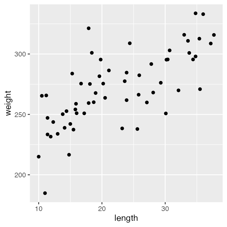


ggplot(dietdata, aes(x = diet, y = weight)) +
  geom_boxplot()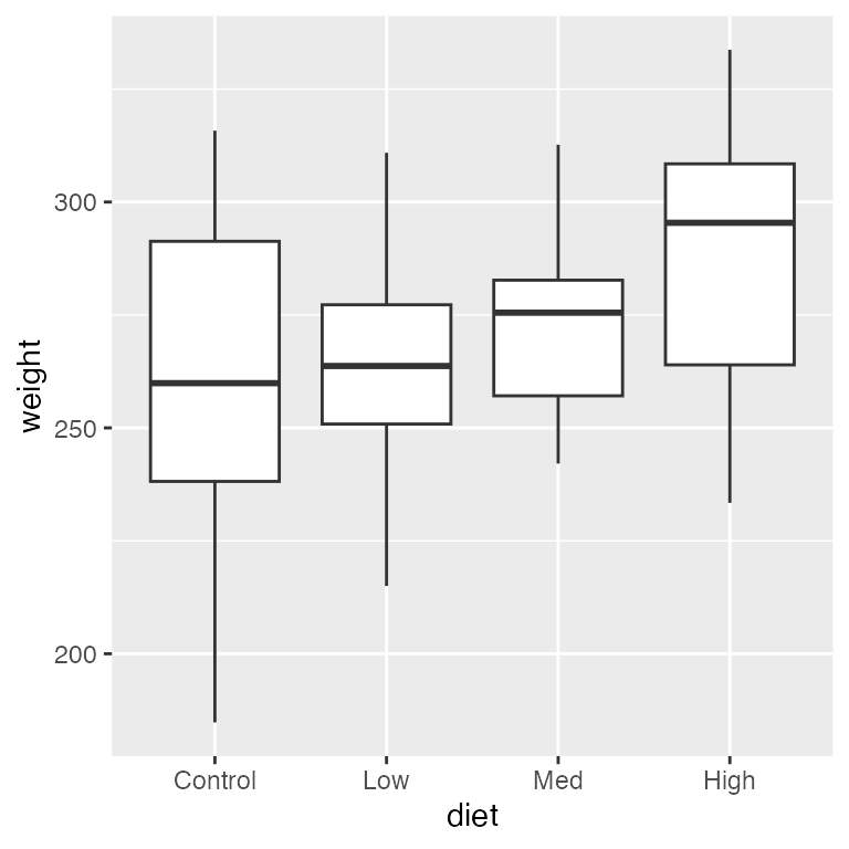

And finally, let’s quantify the relationship between length and weight using a linear regression:

library(knitr)
kable(broom::tidy(fm1), col.names = c("Term", "Estimate", "SE", "Statistic", "p-value"))

Term	Estimate	SE	Statistic	p-value
(Intercept)	213.17440	8.0687929	26.419615	0
length	2.59422	0.3371292	7.695032	0

We can also add regression lines and CIs to our plot using the predict() function:

Create a new data frame containing a sequence of values of the predictor variable length
Predict weight using these values of length
Put predictions and data together for plotting

size <- dietdata$length
nd <- data.frame(length = seq(min(size), max(size), length = 50))
E1 <- predict(fm1, newdata = nd, se.fit = TRUE, interval="confidence")
predictionData <- data.frame(E1$fit, nd)

ggplot() +
  geom_point(data = dietdata, aes(x = length, y = weight)) +
  geom_ribbon(data = predictionData, aes(x = length, ymin = lwr, ymax = upr),
              color = "black", linetype = "longdash", fill = NA) +
  geom_path(data = predictionData, aes(x = length, y = fit))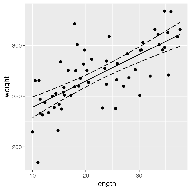

Note that in this simple case, you could use the built in stat_smooth() in ggplot2 to plot the regression line, though that will not always work. predict() is a more general method for creating and plotting regression lines from fitted models.

It’s clear that there is a strong, positive relationship between length and weight. If we want to quantify whether there is an effect of diet on weight, we will clearly need to control for length in our analysis.

As an aside, let’s see what happens if we had ignored length and simply performed a one-way ANOVA.

summary(aov(weight~ diet, data= dietdata))
#>             Df Sum Sq Mean Sq F value Pr(>F)
#> diet         3   5459  1819.6   2.049  0.117
#> Residuals   56  49734   888.1

Notice that we conclude that there is not a difference in weights as a function of diet type even though later in the lab, we will see that diet is an important factor. Why do we reach this incorrect conclusion here?

Now we are ready to perform the ANCOVA. To make interpretation simpler, we will center the continuous predictor.

dietdata$length_centered <- dietdata$length - mean(dietdata$length)
fm2 <- lm(weight~ length_centered + diet, data= dietdata)
summary(fm2)
#> 
#> Call:
#> lm(formula = weight ~ length_centered + diet, data = dietdata)
#> 
#> Residuals:
#>     Min      1Q  Median      3Q     Max 
#> -38.246 -12.180  -2.528  12.152  49.225 
#> 
#> Coefficients:
#>                 Estimate Std. Error t value Pr(>|t|)    
#> (Intercept)     253.9674     4.8751  52.095  < 2e-16 ***
#> length_centered   2.7892     0.2972   9.385 5.16e-13 ***
#> dietLow          13.7271     6.8777   1.996 0.050909 .  
#> dietMed          25.2262     6.9743   3.617 0.000648 ***
#> dietHigh         30.7840     6.8332   4.505 3.50e-05 ***
#> ---
#> Signif. codes:  0 '***' 0.001 '**' 0.01 '*' 0.05 '.' 0.1 ' ' 1
#> 
#> Residual standard error: 18.64 on 55 degrees of freedom
#> Multiple R-squared:  0.6536, Adjusted R-squared:  0.6284 
#> F-statistic: 25.94 on 4 and 55 DF,  p-value: 4.136e-12

How would you interpret each of these parameter estimates in the context of the data?

As before, we can create predictions of weight over a sequences of lengths, for every level of diet:

lengthC <- dietdata$length_centered
nd2 <- data.frame(diet=rep(c("Control", "Low", "Med", "High"), each = 15),
                  length_centered=rep(seq(min(lengthC), max(lengthC),length = 15), times = 4))
E2 <- predict(fm2, newdata=nd2, se.fit = TRUE, interval = "confidence")
predData2 <- data.frame(E2$fit, nd2)

ggplot() +
  geom_point(data = dietdata, aes(x = length_centered, y = weight, color = diet)) +
  geom_line(data = predData2, aes(x = length_centered, y = fit, color = diet)) +
  guides(colour= guide_legend(reverse= T)) +
  scale_y_continuous("Weight") +
  scale_x_continuous("Length")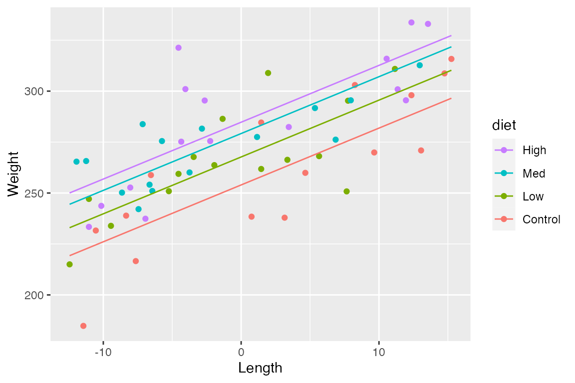

We can also look at multiple comparisons. Note that because we used the lm() function instead of aov(), we are not able to use TukeyHSD() as we did before. Instead we can use glht() function from the multcomp package.

library(multcomp)
summary(glht(fm2, linfct=mcp(diet="Tukey")))
#> 
#>   Simultaneous Tests for General Linear Hypotheses
#> 
#> Multiple Comparisons of Means: Tukey Contrasts
#> 
#> 
#> Fit: lm(formula = weight ~ length_centered + diet, data = dietdata)
#> 
#> Linear Hypotheses:
#>                     Estimate Std. Error t value Pr(>|t|)    
#> Low - Control == 0    13.727      6.878   1.996  0.20188    
#> Med - Control == 0    25.226      6.974   3.617  0.00328 ** 
#> High - Control == 0   30.784      6.833   4.505  < 0.001 ***
#> Med - Low == 0        11.499      6.829   1.684  0.34187    
#> High - Low == 0       17.057      6.819   2.501  0.07083 .  
#> High - Med == 0        5.558      6.871   0.809  0.84997    
#> ---
#> Signif. codes:  0 '***' 0.001 '**' 0.01 '*' 0.05 '.' 0.1 ' ' 1
#> (Adjusted p values reported -- single-step method)

Scenario 2: Blocking

Blocking is used when an additional factor besides our treatment of interest may be contributing to variation in the response variable. While blocking is usually thought of in the context of an ANOVA, it can be used in other linear modeling situations as well.

Blocks can be regions, time periods, individual subjects, etc. but blocking must occur during the design phase of the study. (Later in the course, we will discuss the scenario where we are interested in this second factor and we will no longer refer to it as a block.)

We can write the additive Randomized Complete Block Design as:

\[\large y_{ij} = \mu + \alpha_i + \beta_j + \epsilon_{ij}\]

What would be the hypotheses related to this model?

Blocked ANOVA by hand

To “fit” the RCBD model by hand, we’ll use the gypsy moth data we saw in lecture. In this dataset a researcher has counted the number of caterpillars in each plot treated with either Bt or Dimilin (or left as a control). Additionally, because the treated plots were located in 4 geographic regions, region has been included as a block in the model.

library(FANR6750)
data("mothdata")

head(mothdata)

Region	Treatment	Larvae
1	Control	25
1	Bt	16
1	Dimilin	14
2	Control	10
2	Bt	3
2	Dimilin	2

Before we analyze the moth data, we need to tell R to treat the Treatment and Region variables as factors:

str(mothdata)
#> tibble [12 × 3] (S3: tbl_df/tbl/data.frame)
#>  $ Region   : Factor w/ 4 levels "1","2","3","4": 1 1 1 2 2 2 3 3 3 4 ...
#>  $ Treatment: Factor w/ 3 levels "Control","Bt",..: 1 2 3 1 2 3 1 2 3 1 ...
#>  $ Larvae   : num [1:12] 25 16 14 10 3 2 15 10 16 32 ...

Right now, they are character and integer objects, respectively.

mothdata$Treatment <- factor(mothdata$Treatment, levels = c("Control", "Bt", "Dimilin"))
levels(mothdata$Treatment)
#> [1] "Control" "Bt"      "Dimilin"

mothdata$Region <- factor(mothdata$Region)
levels(mothdata$Region)
#> [1] "1" "2" "3" "4"

Note that we were explicit about the order of levels for Treatment so that control came first.

Means

Next, compute the means:

library(dplyr)

# Grand mean
(grand.mean <- mean(mothdata$Larvae))
#> [1] 14.41667

# Treatment means
(treatment.means <- group_by(mothdata, Treatment) %>% summarise(mu = mean(Larvae)))
#> # A tibble: 3 × 2
#>   Treatment    mu
#>   <fct>     <dbl>
#> 1 Control    20.5
#> 2 Bt         11.8
#> 3 Dimilin    11

# Block means
(block.means <- group_by(mothdata, Region) %>% summarise(mu = mean(Larvae)))
#> # A tibble: 4 × 2
#>   Region    mu
#>   <fct>  <dbl>
#> 1 1       18.3
#> 2 2        5  
#> 3 3       13.7
#> 4 4       20.7

Treatment sums of squares

The formula for the treatment sums of squares:

\[\Large b \times \sum_{i=1}^a (\bar{y}_i - \bar{y}_.)^2\]

b <- nlevels(mothdata$Region)
(SS.treat <- b * sum((treatment.means$mu - grand.mean)^2))
#> [1] 223.1667

Block sums of squares

The formula for the block sums of squares:

\[\Large a \times \sum_{j=1}^b (\bar{y}_j - \bar{y}_.)^2\]

a <- nlevels(mothdata$Treatment)
(SS.block <- a * sum((block.means$mu - grand.mean)^2))
#> [1] 430.9167

Within groups sums of squares

\[\Large \sum_{i=1}^a \sum_{j=1}^b (y_{ij} - \bar{y}_i - \bar{y}_j + \bar{y}_.)^2\]

treatment.means.long <- rep(treatment.means$mu, each = b)
block.means.long <- rep(block.means$mu, times = a)
(SS.within <- sum((mothdata$Larvae - treatment.means.long - block.means.long + grand.mean)^2))
#> [1] 1592.667

NOTE: For the above code to work, treatment.means and block.means must be in the same order as in the original data.

Create ANOVA table

Now we’re ready to create the ANOVA table. Start with what we’ve calculated so far:

df.treat <- a - 1
df.block <- b - 1
df.within <- df.treat*df.block
ANOVAtable <- data.frame(df = c(df.treat, df.block, df.within),
                         SS = c(SS.treat, SS.block, SS.within))
rownames(ANOVAtable) <- c("Treatment", "Block", "Within")
ANOVAtable
#>           df        SS
#> Treatment  2  223.1667
#> Block      3  430.9167
#> Within     6 1592.6667

Next, add the mean squares:

MSE <- ANOVAtable$SS / ANOVAtable$df
ANOVAtable$MSE <- MSE ## makes a new column!

Now, the F-values (with NA for error/within/residual row):

F.stat <- c(MSE[1]/MSE[3], MSE[2]/MSE[3], NA)
ANOVAtable$F.stat <- F.stat

Finally, the p-values

p <- c(1 - pf(F.stat[1], 2, 6), 1 - pf(F.stat[2], 3, 6), NA)
ANOVAtable$p <- p

Quick reminder about calculating p-values

qf(0.95, 2, 6) # 95% of the distribution is below this value of F
#> [1] 5.143253

1-pf(F.stat[1], 2, 6) # Proportion of the distribution beyond this F value
#> [1] 0.6747559

Be sure you understand what each of these functions is doing!

And we’ll display the table using kable(), with a few options to make it look a little nicer:

options(knitr.kable.NA = "") # leave NA cells empty
knitr::kable(ANOVAtable, digits = 2, align = "c",
             col.names = c("df", "SS", "MSE", "F", "p-value"),
             caption = "RCBD ANOVA table calculated by hand")

RCBD ANOVA table calculated by hand
	df	SS	MSE	F	p-value
Treatment	2	223.17	111.58	0.42	0.67
Block	3	430.92	143.64	0.54	0.67
Within	6	1592.67	265.44

Blocked ANOVA using `aov()`

aov1 <- aov(Larvae ~ Treatment + Region, mothdata)
summary(aov1)
#>             Df Sum Sq Mean Sq F value Pr(>F)  
#> Treatment    2  223.2  111.58   5.830 0.0392 *
#> Region       3  430.9  143.64   7.505 0.0187 *
#> Residuals    6  114.8   19.14                 
#> ---
#> Signif. codes:  0 '***' 0.001 '**' 0.01 '*' 0.05 '.' 0.1 ' ' 1

Look what happens if we ignore the blocking variable though:

aov2 <- aov(Larvae ~ Treatment, mothdata)
summary(aov2)
#>             Df Sum Sq Mean Sq F value Pr(>F)
#> Treatment    2  223.2  111.58    1.84  0.214
#> Residuals    9  545.8   60.64

Blocked ANOVA using `lm()`

lm1 <- lm(Larvae~ Treatment + Region, mothdata)
summary(lm1)
#> 
#> Call:
#> lm(formula = Larvae ~ Treatment + Region, data = mothdata)
#> 
#> Residuals:
#>     Min      1Q  Median      3Q     Max 
#> -5.2500 -1.0208  0.1667  0.6042  5.7500 
#> 
#> Coefficients:
#>                  Estimate Std. Error t value Pr(>|t|)    
#> (Intercept)        24.417      3.093   7.893 0.000219 ***
#> TreatmentBt        -8.750      3.093  -2.829 0.030015 *  
#> TreatmentDimilin   -9.500      3.093  -3.071 0.021914 *  
#> Region2           -13.333      3.572  -3.733 0.009705 ** 
#> Region3            -4.667      3.572  -1.306 0.239240    
#> Region4             2.333      3.572   0.653 0.537822    
#> ---
#> Signif. codes:  0 '***' 0.001 '**' 0.01 '*' 0.05 '.' 0.1 ' ' 1
#> 
#> Residual standard error: 4.375 on 6 degrees of freedom
#> Multiple R-squared:  0.8507, Adjusted R-squared:  0.7262 
#> F-statistic: 6.835 on 5 and 6 DF,  p-value: 0.0183

Can you interpret each parameter estimate from the output of aov1 and lm1? What different information is provided from these two ways of constructing the model? Which null hypotheses were rejected? Failed to be rejected?

Assignment

Some time ago, plantations of Pinus caribaea were established at four locations on Puerto Rico. As part of a study, four spacing intervals were used at each location to determine the effect of spacing on tree height. Twenty years after the plantations were established, measurements (height in ft) were made in the study plots. Additionally, soil chemistry was analyzed to determine average pH and nitrogen content (mg N/kg soil) for each tree. Note that although spacing interval is a number, it must be treated as a factor since these 4 spacing intervals (and only these 4) are of interest to the researcher.

You can access these data using:

library(FANR6750)
data("pineData")

Questions/tasks

The researcher would like you to develop several models to investigate the variables affecting tree height in the plantations. When you have done this, she asks that you submit a report of your findings. Instructions for the report are shown below.

Construct a model using the lm() function which predicts tree height as a function of spacing and, because the researcher is also interested in seeing if soil pH is contributing to differences in tree height, include pH as a predictor as well. You may choose to center the continuous variable or not, but remember that it will affect the way you interpret the results.
1. Write out the hypotheses associated with this model
2. Use the equation editor to show the linear model you would use and interpret each term.
3. State your model conclusions in the context of the data. Does there appear to be a relationship between tree height and tree spacing.
4. Determine which tree spacings differ from eachother with regard to their effect on tree height.
5. Create a publication quality plot displaying the effect that pH and tree spacing has on tree height. The figure should have a descriptive caption and any aesthetics (color, line type, etc.) should be clearly defined.
Construct an ANOVA table by hand which shows the relationship between tree height and spacing as well as the other categorical variable of location. The researcher is not particularly interested in geographic location and she’s not sure of the exact mechanism, but she thinks it may affect the results.
1. Create a well formatted ANOVA table with a table header using available R functions.
2. Was it necessary to include location in your model? Would it have changed your overall conclusions about the effect of spacing on tree height if you had not included it?
Construct a model using the lm() function that predicts tree height as a function of soil pH and nitrogen content.
1. Write out the hypotheses associated with this model
2. Use the equation editor to show the linear model you would use and interpret each term.
3. Interpret each parameter estimate in the model output
Discussion: Up to now, we have discussed how we might construct several types of models which are all being used to predict tree height in this data scenario. Later in the semester we will talk about ‘model selection’ which is the process of choosing one model out of several that somehow best represents the research system. Having no formal instruction on this topic yet (or perhaps you do) explain how you think model selection might be done. What kinds of metrics might you use to decide which model best represents the data? (There is no one right answer here and all reasonably thought out answers will be accepted.)

You may format the report however you like but it should be well-organized, with relevant headers, plain text, and the elements described above.

As always:

Be sure the output type is set to: output: html_document
Be sure to set echo = TRUE in all R chunks
See the R Markdown reference sheet for help with creating R chunks, equations, tables, etc.
See the “Creating publication-quality graphics” reference sheet for tips on formatting figures

Under the hood, R actually treats factors as integers - 1, 2, 3… - with character labels for each level↩︎

FANR 6750: Experimental Methods in Forestry and Natural Resources Research

Fall 2023

Lab 5

Today’s topics

Scenarios

Scenario 1: ANCOVA

Data example

An aside about factors

Back to the data

Scenario 2: Blocking

Blocked ANOVA by hand

Means

Treatment sums of squares

Block sums of squares

Within groups sums of squares

Create ANOVA table

Blocked ANOVA using `aov()`

Blocked ANOVA using `lm()`

Assignment

Lab 6: Multiple Regression

FANR 6750: Experimental Methods in Forestry and Natural Resources Research

Fall 2023

Lab 5

Today’s topics

Scenarios

Scenario 1: ANCOVA

Data example

An aside about factors

Back to the data

Scenario 2: Blocking

Blocked ANOVA by hand

Means

Treatment sums of squares

Block sums of squares

Within groups sums of squares

Create ANOVA table

Blocked ANOVA using aov()

Blocked ANOVA using lm()

Assignment

Blocked ANOVA using `aov()`

Blocked ANOVA using `lm()`