LECTURE 3: principles of statistical inference
Outline
1) Uncertainty in statistical models
2) Sampling distributions
\[\Large Statistics = Information + Uncertainty\]
In the last lecture, we learned that models allow us to quantify relationships between variables based on samples
We also learned that sampling = uncertainty
- Parameter estimates from samples will never exactly equal population parameters
Inference about populations requires quantifying the magnitude of this uncertainty
But how can we measure how far our estimates are from the population parameters if we don’t know the population parameters?
Parameters vs statistics
Parameters
- Attributes of the population
- Mean ( \(\mu\) )
- Variance ( \(\sigma^2\) )
- Standard deviation ( \(\sigma\) )
- Usually unknown
- Parameters are the quantities of interest
- Generally denoted using Greek letters
Statistics
- Attributes of the sample
- Mean ( \(\bar{y}\) or \(\hat{\mu}\) )
- Variance ( \(s^2\) or \(\hat{\sigma}^2\) )
- Standard deviation ( \(s\) or \(\hat{\sigma}\) )
Sampling error
Question: What is the probability that \(\bar{y} = \mu\)?
- Fact: The sample mean will never equal the population mean
- The difference between \(\bar{y}\) and \(\mu\) is sampling error
- Sampling error can be reduced but it cannot be eliminated
Problem: If we don’t know \(\mu\), how do we know how far our estimate is from the true value?
- Answer: We don’t (for any specific sample)
- BUT…we do know how far, on average, a sample of size \(n\) will be from the true value
The sampling distribution
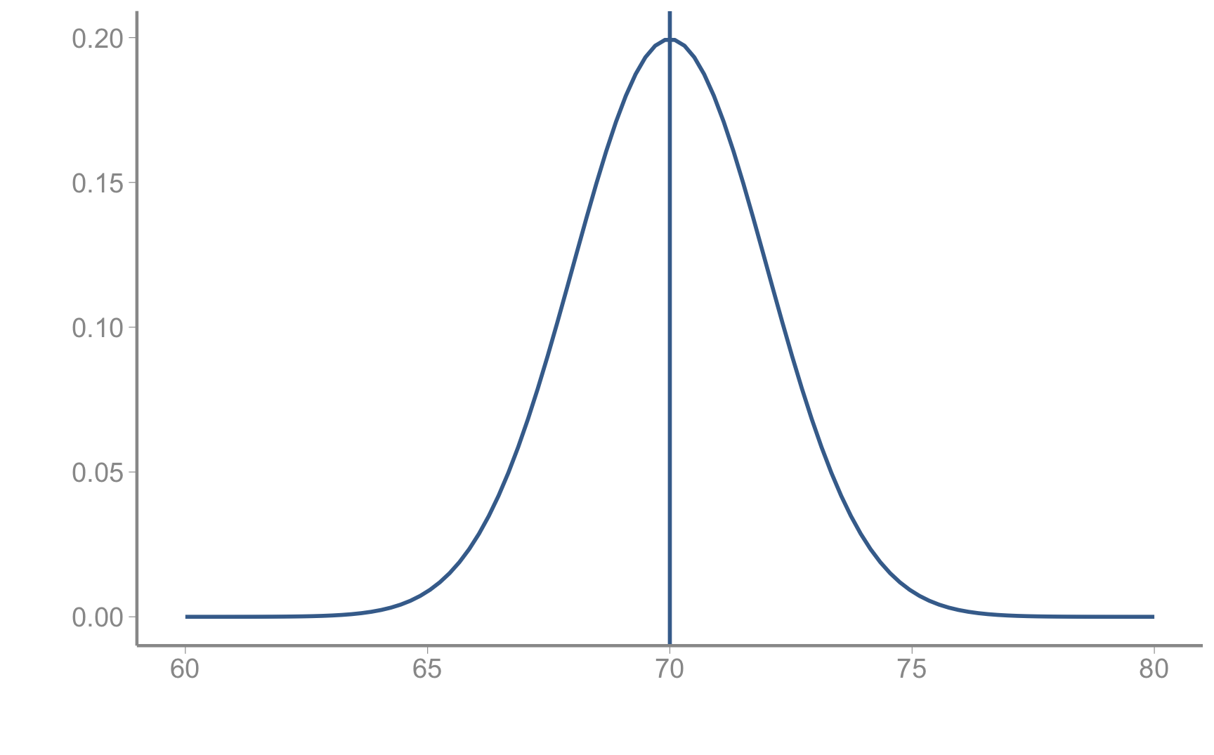
A population
![]()
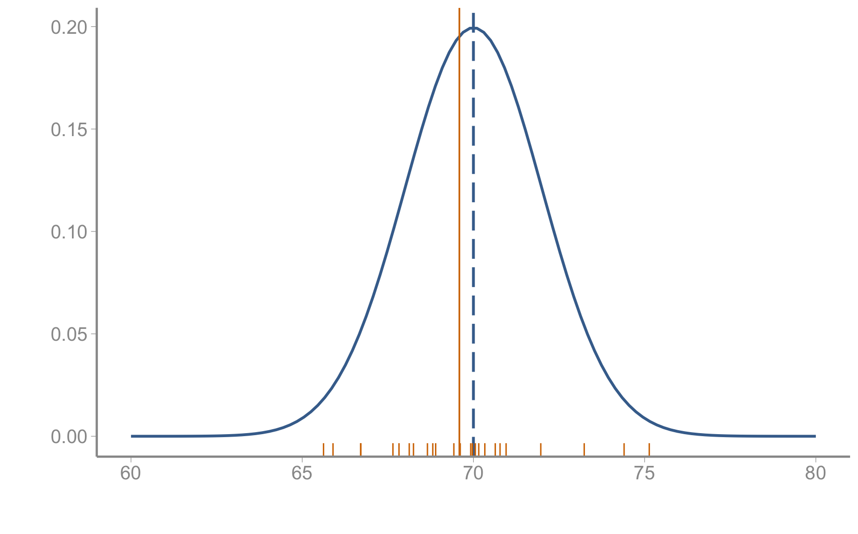
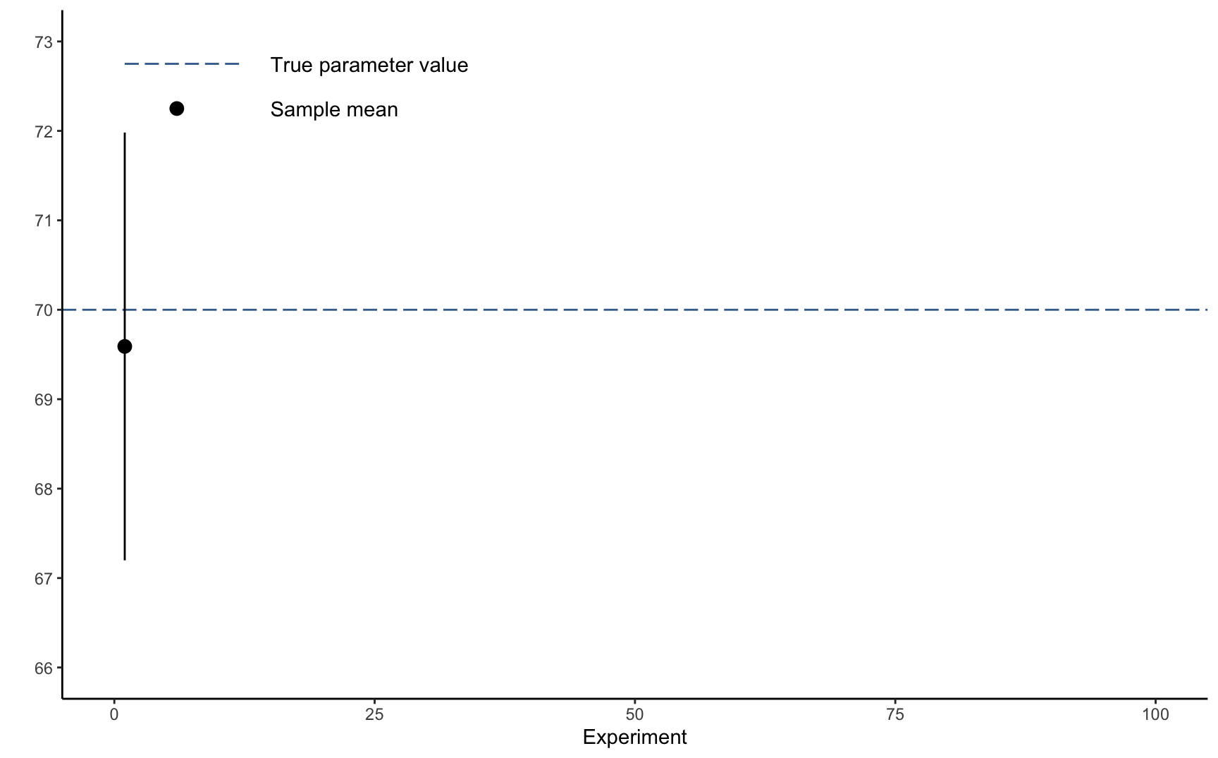
A single sample (n = 25)
![]()
A single sample (n = 25)
![]()
Standard deviation
![]()
This error bar is the standard deviation of our sample!
Standard deviation
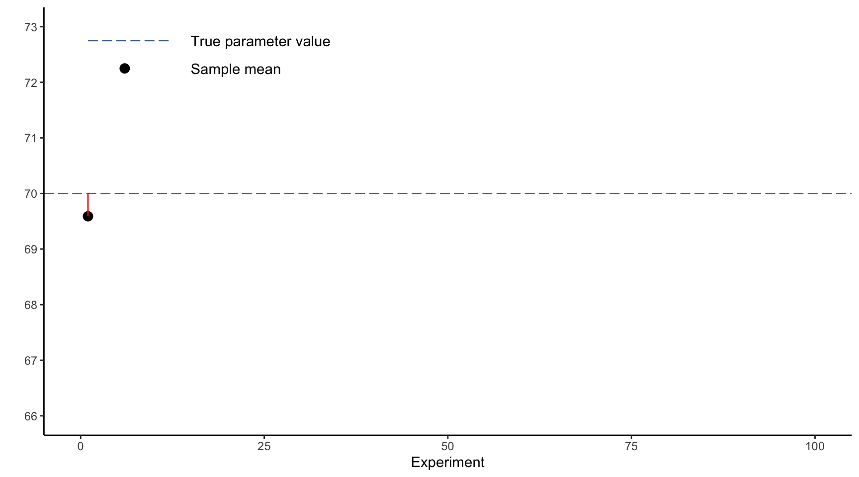
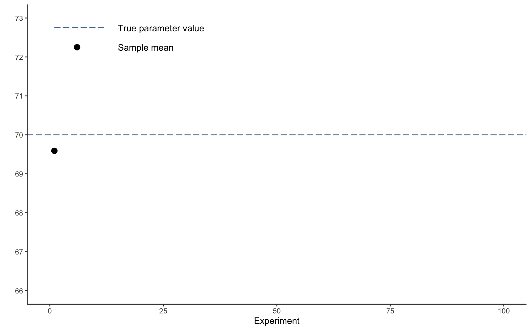
But remember, what we really want to know is, how far is the sample mean from the true parameter value?
The sampling distribution
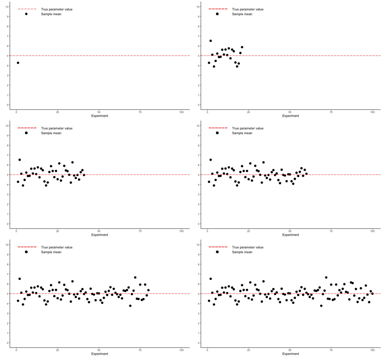
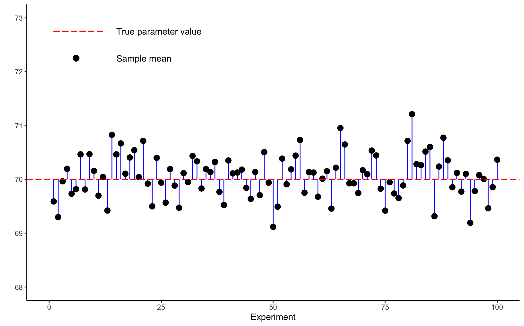
Imagine we could repeat our experiment many, many times
![]()
the sampling distribution
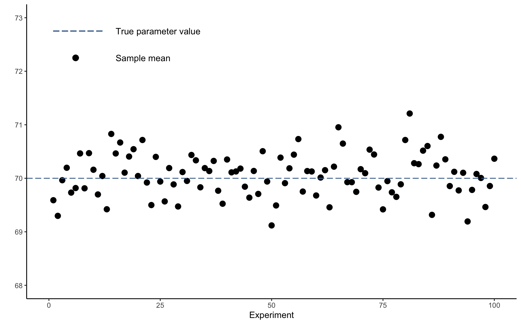
The collection of sample means is referred to as the sampling distribution
![]()
The sampling distribution
The collection of sample means is referred to as the sampling distribution
![]()
The sampling distribution
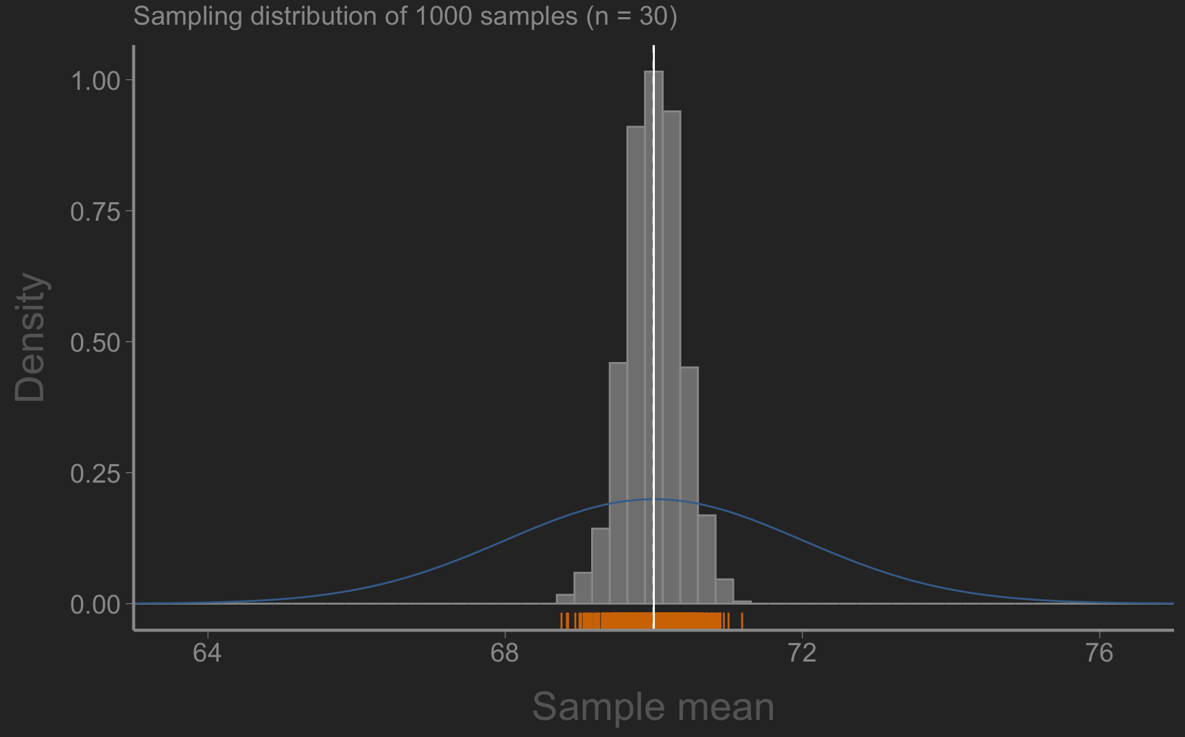
The standard deviation of the sampling distribution measures, on average, how far each sample mean from the true population value
![]()
The sampling distribution
We rarely repeat experiments
But we can estimate the standard deviation of the sampling distribution from a single sample!
How? The central limit theorem!
Central limit theorem
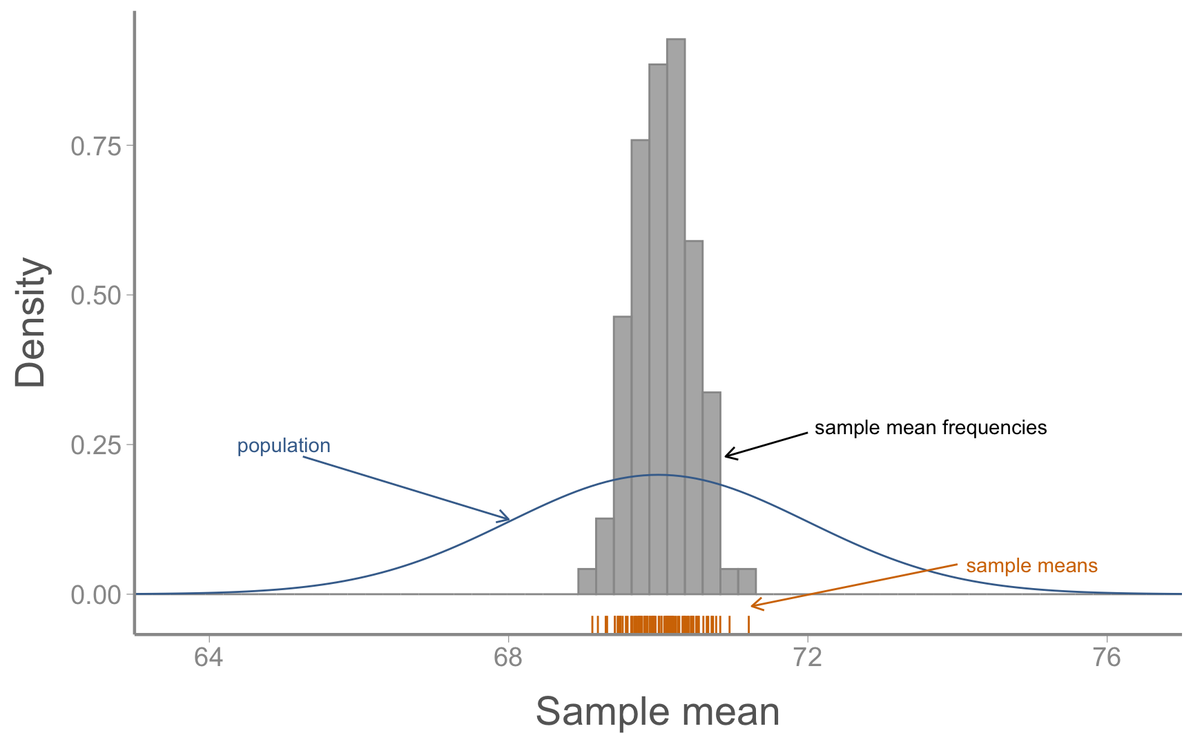
For a population with mean \(\mu\) and standard deviation \(\sigma\), the sampling distribution will be (approximately) normally distributed with mean \(\mu_X = \mu\) and standard deviation \(\sigma_X = \sigma/\sqrt{n}\).
![]()
Central limit theorem
For a population with mean \(\mu\) and standard deviation \(\sigma\), the sampling distribution will be (approximately) normally distributed with mean \(\mu_X = \mu\) and standard deviation \(\sigma_X = \sigma/\sqrt{n}\).
This might seem academic but it is hugely important
given sufficient sample size ( \(\sim n > 30\) ), we know the sampling distribution will be normally distributed without needing to repeat the experiment
although we never know the true population mean \(\mu\), we can estimate how far (on average) our sample mean is likely to be away from it (that’s what the standard deviation is!)
the CLT will hold true regardless of whether the source population is normal!
Demonstration using simulations
Standard error
The standard deviation of the sampling distribution is called the standard error of the mean (or just the standard error)
\[\Large SE =\frac{s}{\sqrt{n}}\]
Descriptive vs inferential statistics
The sample standard deviation ( \(s\) ) is a descriptive statistic
\[\large s = \sqrt{s^2}\]
- \(s\) tells us how far, on average, each observation \(y\) is from the sample mean \(\bar{y}\)
The standard error (SE) is an inferential statistic
\[\large SE = \frac{s}{\sqrt{n}}\]
- \(SE\) tells us how far, on average, each sample mean \(\bar{y}\) is from the population mean \(\mu\)
Quick review
- Sampling is a stochastic process
- Sample statistics (mean, standard deviation) will vary from sample to sample
- The sampling distribution is an (imaginary) collection of statistics from repeated samples of the same population
- Assumes that the procedure for generating samples (e.g., sample size) is identical
- Standard error is the standard deviation of the sampling distribution
We will explore these concepts in lab, using R to generate and visualize repeated samples, calculate properties of the sampling distribution
Confidence intervals
Uncertainty is commonly reported using confidence intervals
- this is a concept that seems intuitive but in reality it is commonly misunderstood
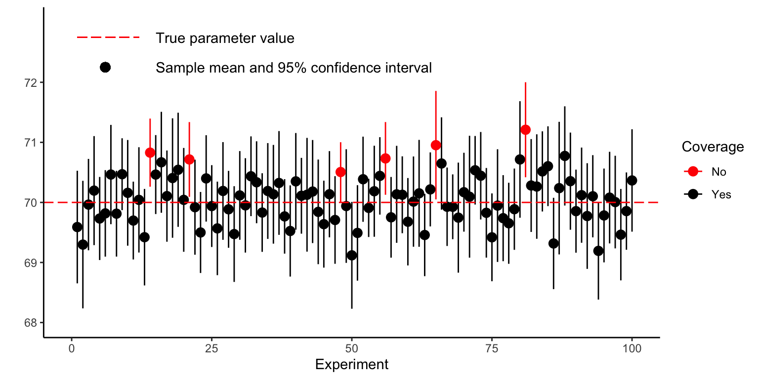
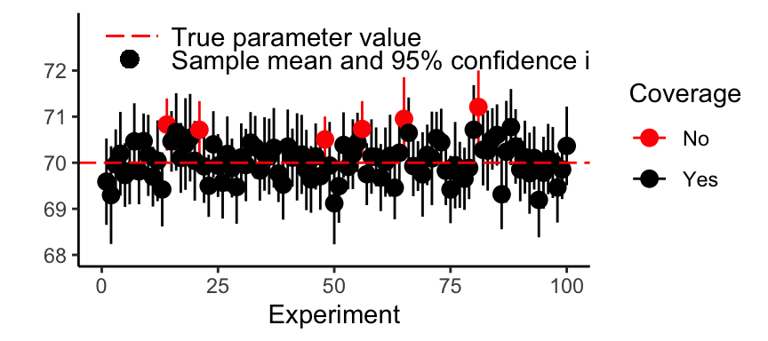
If we calculated a \(x\)% confidence interval from repeated samples of the population, about \(x\)% of those confidence intervals would contain the true population mean
![]()
Calculating confidence intervals
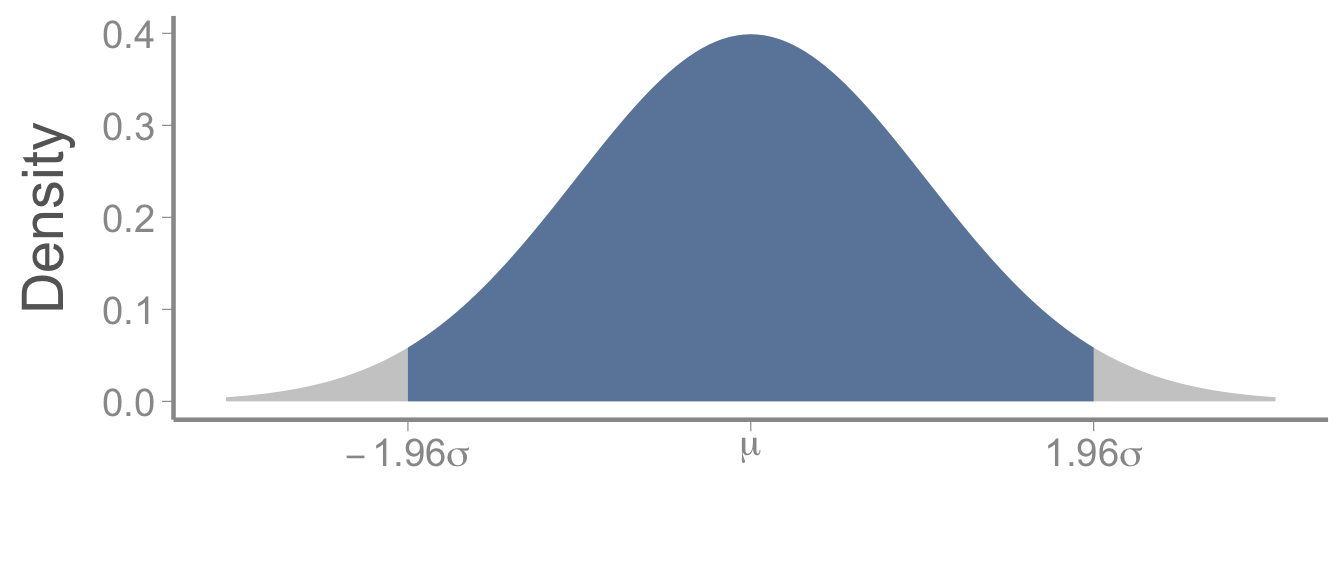
95% of a normal distribution falls between -1.96 and 1.96 standard deviation of the mean
Question - if this is the sampling distribution, what is the standard deviation? What is our estimate of the mean?
95% CI = \(\large \bar{y} \pm 1.96 \times SE\)
Confidence intervals
What a confidence interval is NOT:
- “there is an \(x\)% probability that the true population parameter is inside this interval”
The true population value is considered a fixed parameter
Before we collect our sample, the ends of the confidence intervals are considered random variables (i.e., their value will change each time we collect a sample)
- Like all random variables, we can describe the long-term (i.e., asymptotic) expectations of confidence intervals if we repeated the experiment many times
After we collect our sample, the confidence interval either does or does not contain the true population value
Confidence intervals
Think of confidence intervals like trying to determine where the stake is in a game of horseshoes by looking at where the horseshoes landed
The true parameter (i.e., the stake) does not move
Each horseshoe is the CI based on a single sample (i.e., one throw)
Before a horseshoe is thrown, there is some probability it will land around the stake
After it is thrown, it is either around the stake or not
or…
Confidence intervals
I like to think of confidence intervals as providing a range of values that, based on our sample, are consistent with the population mean (plausible interval?)
- If want to be more confident that the CI contains the parameter (e.g., 50% CI vs 95% CI), what happens to the size of the interval?
The confidence interval we calculate from our sample will not include the true population mean 1 - \(x\)% of the time
Of course, with our real data, we have no way of knowing if our sample is one of the black points on this graph 😀 or one of the red dots 😭
For thought
If our goal is generally to decrease uncertainty in parameter estimates:
- What factors determine the magnitude of our uncertainty estimates (SE or confidence intervals)?
- What can we, as researchers, control when we design experiments to minimize uncertainty? What can we not control?
Looking ahead
Next time: Linear models part 1: categorical predictor w/ 2 levels
Reading: Fieberg chp. 3.6