LECTURE 4: linear models part 1: categorical predictor w/ 2 levels

Outline

1) Motivation

2) Categorical predictor with 1 level (linear model vs t-test formulations)

3) Categorical predictor with 2 levels (linear model vs t-test formulations)

Motivation

In lecture 2, we discussed linear models as a flexible way to quantify relationships between variables

\[y_i = \beta_0 + \beta_1 * x_i + \epsilon_i\] \[\epsilon_i \sim normal(0, \sigma)\]

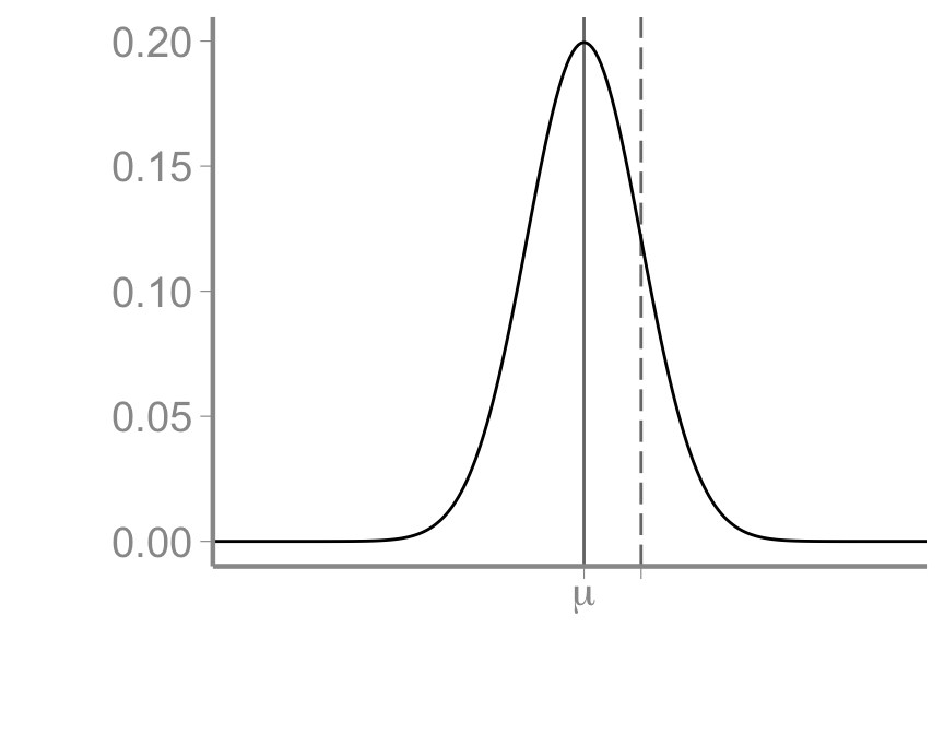
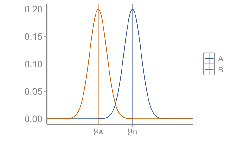
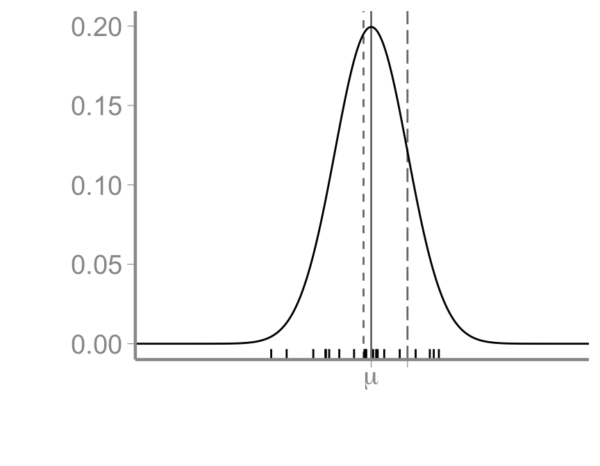
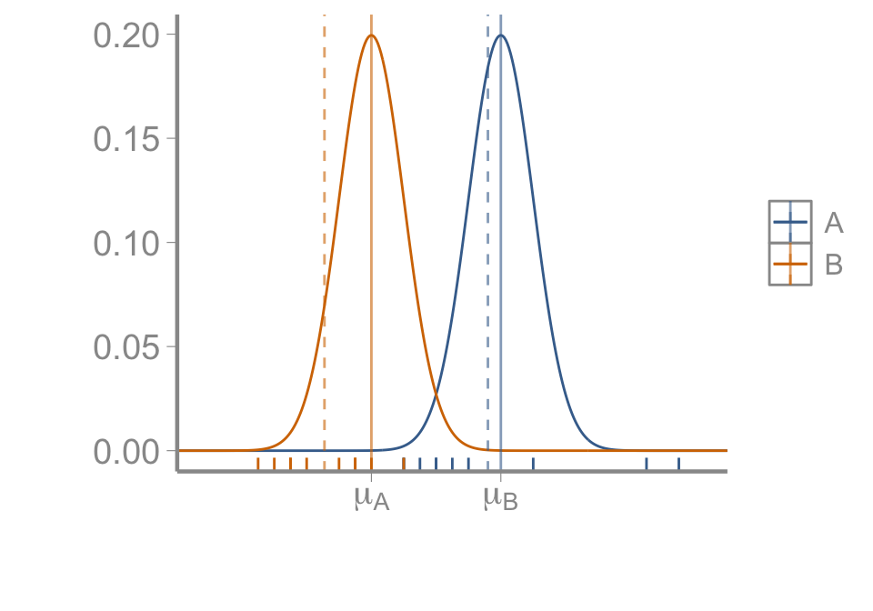
In lecture 3, we discussed sampling and statistical inference

• Samples allow us to estimate population parameters but also introduce error due to the random nature of sampling

• Standard errors and confidence intervals allow us to quantify the magnitude of sampling error

In this lecture, we will put these concepts into practice by fitting and interpreting simple linear models

Motivation

One common research objective is to determine whether the mean of a population differs from some specific value or whether the mean of two populations differ from each other

• Is the average size of hatchery-raised fish above the threshold needed for release?

• Does a newly developed plant variety have better disease resistance than the current variety?

• Does taking FANR6750 improve students’ statistical knowledge compared to students who don’t take FANR6750?

Although these may seem like simple questions, answering them still requires statistical models. Why?

Populations and samples

The questions on the previous slide ask whether a population mean differs from a specific value or another population’s mean

But remember, we don’t know the population means. They has to be estimated. How?

Populations and samples

The questions on the previous slide ask whether a population mean differs from a specific value or another population’s mean

But remember, we don’t know the population means. They has to be estimated. How?

• By sampling!

Statistical inference

• Our best estimates of the population means are the sample means

• But we know the sample means will never equal the population means

• Because of the uncertainty caused by this sampling error, answering even these simple questions requires statistical models

• In this lecture, we will learn to formulate these questions as linear models

  • Fortunately, the models used for these examples are relatively simple

  • Although simple, the models in this lecture will serve as the foundation for all of the more complex models we will use later in the semester

  • This lecture will focus on model structure and interpretation of parameters. Later lectures will focus on using model output for inference about population parameters

Example 1

We are interested in whether a certain brand of scale provides accurate mass measurements

Hypothesis

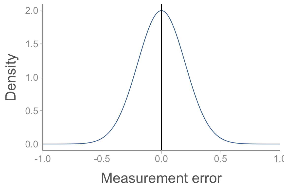
Measurement error, measured as the difference between the mass indicated by the scale and the true mass of an object, is 0 (on average)

Example 1

Data collection:

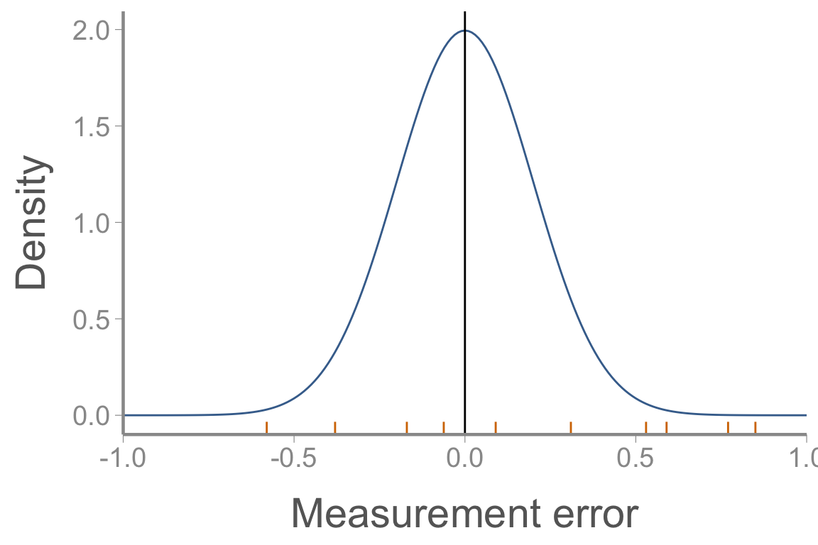
• Randomly sample 10 scales of the same make and model

• Weigh a test object (of known mass) on each scale and record the difference between the measured and true mass

Data:

-0.062, -0.38, 0.85, -0.58, 0.53, 0.09, 0.31, 0.77, 0.59, -0.17

The linear model

\[y_i = \beta_0 + \epsilon_i\]

\[\epsilon_i \sim normal(0, \sigma)\]

• \(\beta_0\) is the expected (or average) measurement error across all scales

• \(\epsilon_i\) is residual error associated with each measurement

• This is most simple linear model we can construct

• If our hypothesis is correct, \(\beta_0 = 0\)

Question: What is the value of \(\beta_0\) if our hypothesis is wrong?

Summary statistics

Data:

y <- c(-0.062, -0.38, 0.85, -0.58,  0.53,  0.09,  0.31,  0.77,  0.59,  -0.17)

\(\large \bar{y}\)

mean(y)

[1] 0.1948

\(\large s\)

sd(y)

[1] 0.4925

SE

sd(y)/sqrt(10)

[1] 0.1557

Visualizing the data

Visualizing the data

The linear model

Because this is a linear model, we can fit it using the lm function:¹

fit1 <- lm(y ~ 1)

summary(fit1)

Call:
lm(formula = y ~ 1)

Residuals:
    Min      1Q  Median      3Q     Max 
-0.7748 -0.3378  0.0052  0.3802  0.6552 

Coefficients:
            Estimate Std. Error t value Pr(>|t|)
(Intercept)    0.195      0.156    1.25     0.24

Residual standard error: 0.492 on 9 degrees of freedom

• The (Intercept) estimate corresponds to \(\beta_0\) (look familiar?)

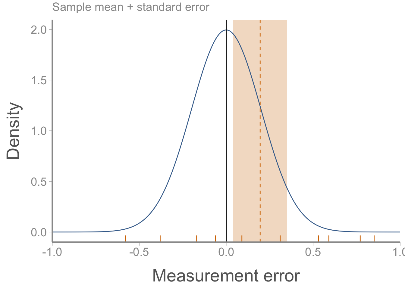
• The standard error calculated by R is the same as we calculated by hand

• We will discuss whether there is evidence that \(\beta_0 \neq 0\) in the next lecture

• Congratulations, you fit your first linear model in R²

The linear model as a t-test

The model we just fit has a corresponding “test” that you may encounter: the one-sample t-test

• One-sample t-tests are used to test whether the mean of a population differs from some value (in this case 0)

R has a built-in function to fit t-tests:³

t.test(y, mu = 0)

    One Sample t-test

data:  y
t = 1.3, df = 9, p-value = 0.2
alternative hypothesis: true mean is not equal to 0
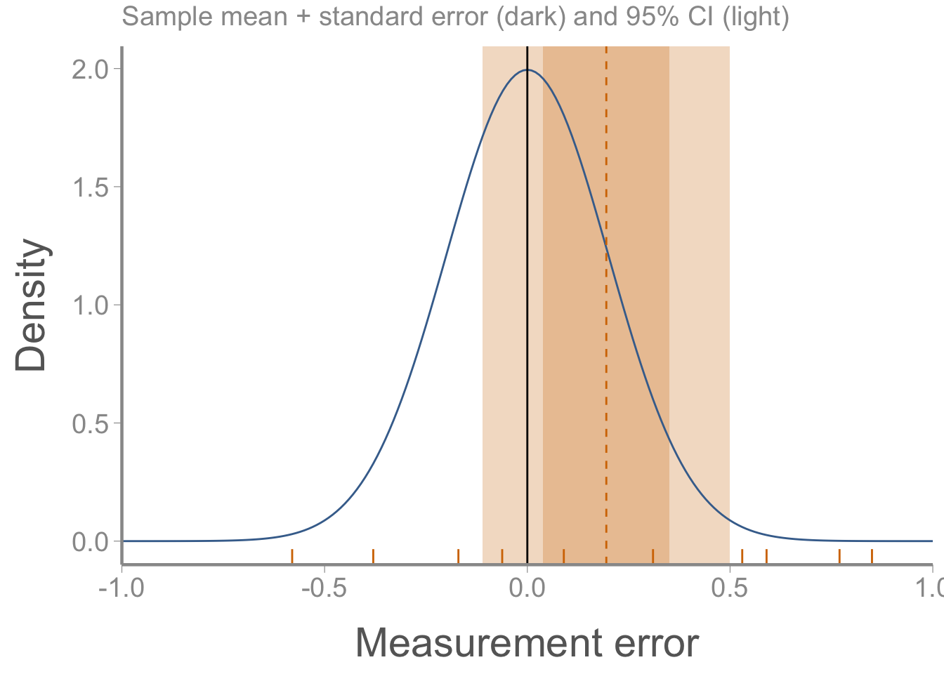
95 percent confidence interval:
 -0.1575  0.5471
sample estimates:
mean of x 
   0.1948 

• Note that the mean (and the SE, t-statistic, p-value, confidence intervals) are exactly the same in both approaches

The one-sample t-test by hand

Because this is such a simple model, we can calculate \(\beta_0\) and the standard error by hand very easily

(beta0 <- mean(y))

[1] 0.1948

(SE <- sd(y)/sqrt(10))

[1] 0.1557

Again, we will discuss how to use this information to determine whether \(\beta_0\) is or is not equal to 0 in another next lecture

But that is it - the first model of the semester (fit three ways - lm(), t.test(), and by hand)

Example 2

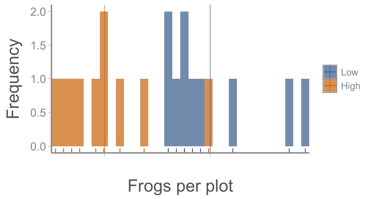
We are interested in determining how urban development influences the abundance of strawberry poison-dart frog (Oophaga pumilio)

Hypothesis:

Strawberry frog abundance will differ between islands with high urban development and islands with low urban development

Example 2

Field procedure:

• \(n=10\) plots are established on one high-development island and one low-development island

• Within each plot, strawberry frogs are counted within 5 randomly-located quadrats

Data:

Low development: 16, 14, 18, 17, 29, 31, 14, 16, 22, 15

High development: 2, 11, 6, 8, 0, 3, 19, 1, 6, 5

Example 2

Fitting the model in R

data(frogdata)

fit <- lm(Frogs ~ Development, data = frogdata)

summary(fit)

Call:
lm(formula = Frogs ~ Development, data = frogdata)

Residuals:
   Min     1Q Median     3Q    Max 
 -6.10  -4.12  -1.70   2.12  12.90 

Coefficients:
                Estimate Std. Error t value Pr(>|t|)    
(Intercept)        19.20       1.87   10.29  5.7e-09 ***
DevelopmentHigh   -13.10       2.64   -4.97    1e-04 ***
---
Signif. codes:  0 '***' 0.001 '**' 0.01 '*' 0.05 '.' 0.1 ' ' 1

Residual standard error: 5.9 on 18 degrees of freedom
Multiple R-squared:  0.578, Adjusted R-squared:  0.555 
F-statistic: 24.7 on 1 and 18 DF,  p-value: 1e-04

• In this example, R returns two parameter estimates: (Intercept) and DevelopmentHight

• To interpret this output, we need to know how R codes categorical predictors…

Quick review

A “simple” linear model

\[\underbrace{\LARGE E[y_i] = 7 + 3.5 \times x_i}_{Deterministic}\]

Quick review

A “simple” linear model

\[\underbrace{\LARGE E[y_i] = 7 + 3.5 \times x_i}_{Deterministic}\]

\[\underbrace{\LARGE y_i \sim normal(E[y_i], \sigma=0.25)}_{Stochastic}\]

The linear model

Same model, different \(\Large x\)

\[\underbrace{\LARGE E[y_i] = 7 + 3.5 \times x_i}_{Deterministic}\]

The linear model

Same model, different \(\Large x\)

\[\underbrace{\LARGE E[y_i] = 7 + 3.5 \times x_i}_{Deterministic}\]

\[\underbrace{\LARGE y_i \sim normal(E[y_i], \sigma=0.25)}_{Stochastic}\]

The linear model

\[\LARGE E[y_i] = \beta_0 + \beta_1 x_i\]

When \(x = 0\):

• \(E[y] = \beta_0\)

• What is the interpretation of \(\beta_0\)?

When \(x = 1\):

• \(E[y] = \beta_0 + \beta_1\)

• What is the interpretation of \(\beta_1\)?

Categorical predictors in R

When you include a categorical predictor (factor or character object) in your model, R recodes it is a dummy variable

• For a predictor with two levels, one level gets coded as \(0\) and the other as \(1\)

• For unordered factors or character objects, levels are determined by alphabetical order

• For ordered factors, levels are determined by factor levels

str(frogdata)

'data.frame':   20 obs. of  2 variables:
 $ Frogs      : num  16 14 18 17 29 31 14 16 22 15 ...
 $ Development: Factor w/ 2 levels "Low","High": 1 1 1 1 1 1 1 1 1 1 ...

Fitting the model in R

data(frogdata)

fit2 <- lm(Frogs ~ Development, data = frogdata)

broom::tidy(fit2)

# A tibble: 2 × 5
  term            estimate std.error statistic       p.value
  <chr>              <dbl>     <dbl>     <dbl>         <dbl>
1 (Intercept)         19.2      1.87     10.3  0.00000000573
2 DevelopmentHigh    -13.1      2.64     -4.97 0.000100     

• The (Intercept) estimate (\(\beta_0\)) is the expected number of frogs in a low-development plot

• The DevelopmentHigh estimate (\(\beta_1\)) is the difference between low-development and high-development plots

Question: Are there fewer frogs in high-development plots?

Fitting the model by hand

In this case, we can also fit the model “by hand”

The parameter estimates are:

mu_high <- mean(frogdata$Frogs[frogdata$Development == "High"])
mu_low <- mean(frogdata$Frogs[frogdata$Development == "Low"])

(beta_0.hat <- mu_low)

[1] 19.2

(beta_1.hat <- mu_high - mu_low)

[1] -13.1

How do we calculate the standard errors?

Fitting the model by hand

How do we calculate the standard errors?

Because we have samples from two populations (low and high development), we have to use the pooled variance of both samples to calculate the correct standard errors:

\[\large s^2_p = \frac{(n_L − 1)s^2_L + (n_H − 1)s^2_H}{n_L + n_H − 2}\]

var_low <- var(frogdata$Frogs[frogdata$Development == "Low"])
var_high <- var(frogdata$Frogs[frogdata$Development == "High"])

# Pooled variance
(s2.p <- (9*var_low + 9*var_high)/18)

[1] 34.81

Fitting the model by hand

How do we calculate the standard errors?

With the pooled variance calculated, we can calculate the standard errors. For the intercept:

\[SE_{\beta_0} = \sqrt{\frac{s^2_p}{n_L}}\]

[1] 1.866

For the slope:

\[SE_{\beta_1} = \sqrt{\frac{s^2_p}{n_L} + \frac{s^2_p}{n_H}}\]

[1] 2.638

What is the interpretation of these standard errors?

The linear model as a t-test

As before, the model we just fit has a corresponding “test” that you may encounter: the two-sample t-test

t.test(Frogs ~ Development, data = frogdata)

    Welch Two Sample t-test

data:  Frogs by Development
t = 5, df = 18, p-value = 1e-04
alternative hypothesis: true difference in means between group Low and group High is not equal to 0
95 percent confidence interval:
  7.554 18.646
sample estimates:
 mean in group Low mean in group High 
              19.2                6.1 

• Used to test whether the means of two population are different

• Results are exactly the same as lm

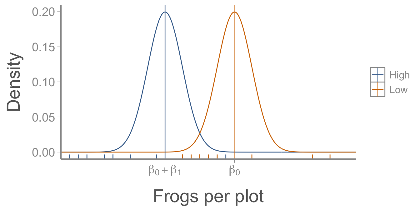
Visualizing the linear model

Other ways to fit the model

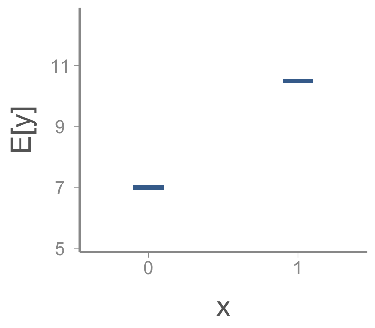
By default, the linear model approach provides the mean of the reference group and the difference in the group means

• This version of the linear model formulation is usually referred to as the effects parameterization

• We can easily calculate the mean of group 2 from the linear model as \(\beta_0 + \beta_1\)

• We can also recode the model in R to provide the group means (the means parameterization)

fit3 <- lm(Frogs ~ Development - 1, data = frogdata)
broom::tidy(fit3)

# A tibble: 2 × 5
  term            estimate std.error statistic       p.value
  <chr>              <dbl>     <dbl>     <dbl>         <dbl>
1 DevelopmentLow      19.2      1.87     10.3  0.00000000573
2 DevelopmentHigh      6.1      1.87      3.27 0.00426      

Summary

• The simplest linear model we can construct tests whether the mean of a sample is different from some null value (usually 0)

  • This model is the same as a one-sample t-test

• The same linear model can be extended to test whether the mean of two groups differ from each other

  • The lm() function uses dummy variables, i.e., coding one treatment level as 0 and the other as 1

  • By default, the intercept is the mean of the reference group and the slope parameter is the difference between the group means

  • This model is the same as a two-sample t-test

• The alternative ways to fit this model (t-test, effects parameterization, means parameterization) provide the exact same information

  • In other words, they do not change your conclusions!

Looking ahead

Next time: Null hypothesis testing

Reading: Fieberg chp. 1.10

Footnotes

1. In R’s formula syntax, a linear model that contains only an intercept value is written by putting a 1 on the right hand side of the formula. The summary() function is used to print the output of the fitted model

2. Simple, right?

3. The mu argument is used to specify the null value we want to compare the population mean to. The default is 0, so adding the mu = 0 argument is not necessary in this case, but was included so demonstrate how to test values other than 0