LECTURE 6: evaluating linear model assumptions

Outline

1) Review of linear model assumptions

2) Evaulating assumptions

3) Robustness to assumption violations

Assumptions

EVERY model has assumptions

• Assumptions are necessary to simplify real world to workable model

• If your data violate the assumptions of your model, inferences may be invalid

• Always know (and test) the assumptions of your model

Linear model assumptions

\[\large y_i = \beta_0 + \beta_1 x_i + \epsilon_i\]

\[\large \epsilon_i \sim normal(0, \sigma)\]

1. Linearity: The relationship between \(x\) and \(y\) is linear

2. Normality: The residuals are normally distributed

3. Homogeneity: The residuals have a constant variance at every level of \(x\)

4. Independence: The residuals are independent (i.e., uncorrelated with each other)

Evaluating assumptions

Evaluating whether your data violate the linear model assumptions relies heavily on residuals

• Residuals are the difference between the observed and predicted response value of each observation

  • \(r_i = (y_i - \hat{y}_i)\)

• Plotting the residuals vs the predicted values provides a visual assessment of the linearity assumptions

• Plotting the residuals vs the predicted values or \(X\) provides a visual assessment of the variance assumption

• Plotting a Q-Q plot or histogram of the residuals provides visual assessments of the normality assumption

Evaluating assumptions

Fortunately, multiple R packages include functions for making diagnostic plots from a fitted lm object

library(performance)
data("biomassdata")
fm1 <- lm(biomass ~ elevation + rainfall, data = biomassdata)
check_model(fm1, check = c("linearity", "homogeneity", "qq", "normality"))

Linearity

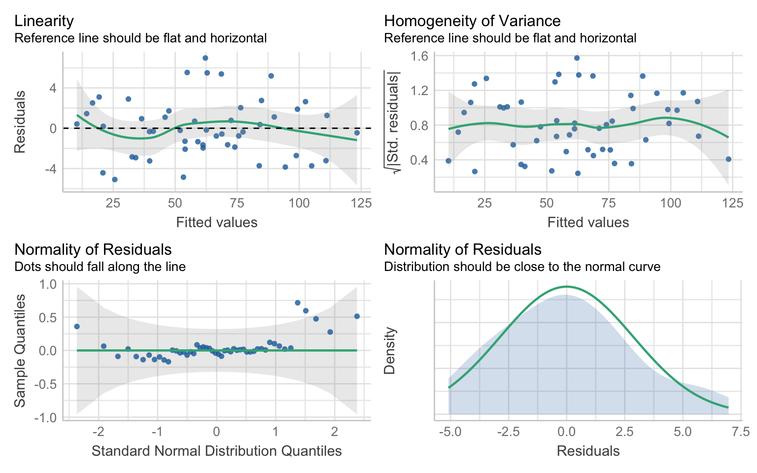
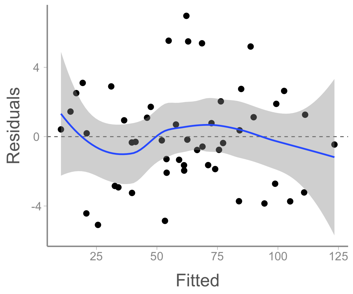
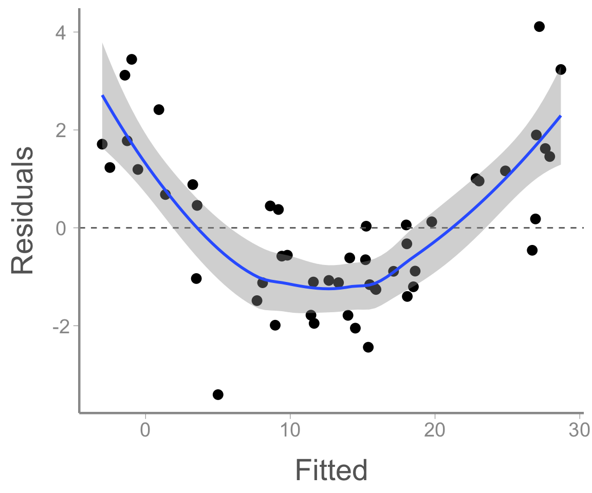
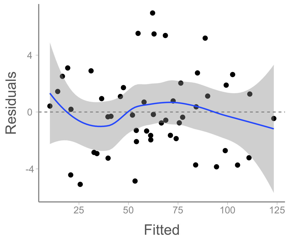
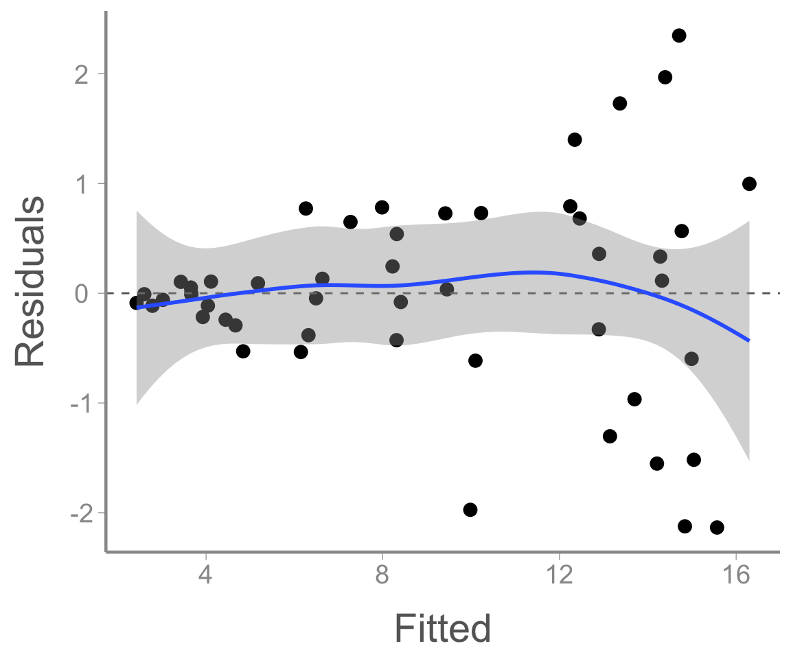
Deviations from linearity will appear as patterns in the residual plot

Homogeneity of variance

Heteroscedasticity will appear as patterns (often funnel-shaped) in the residual plot

Homogeneity of variance

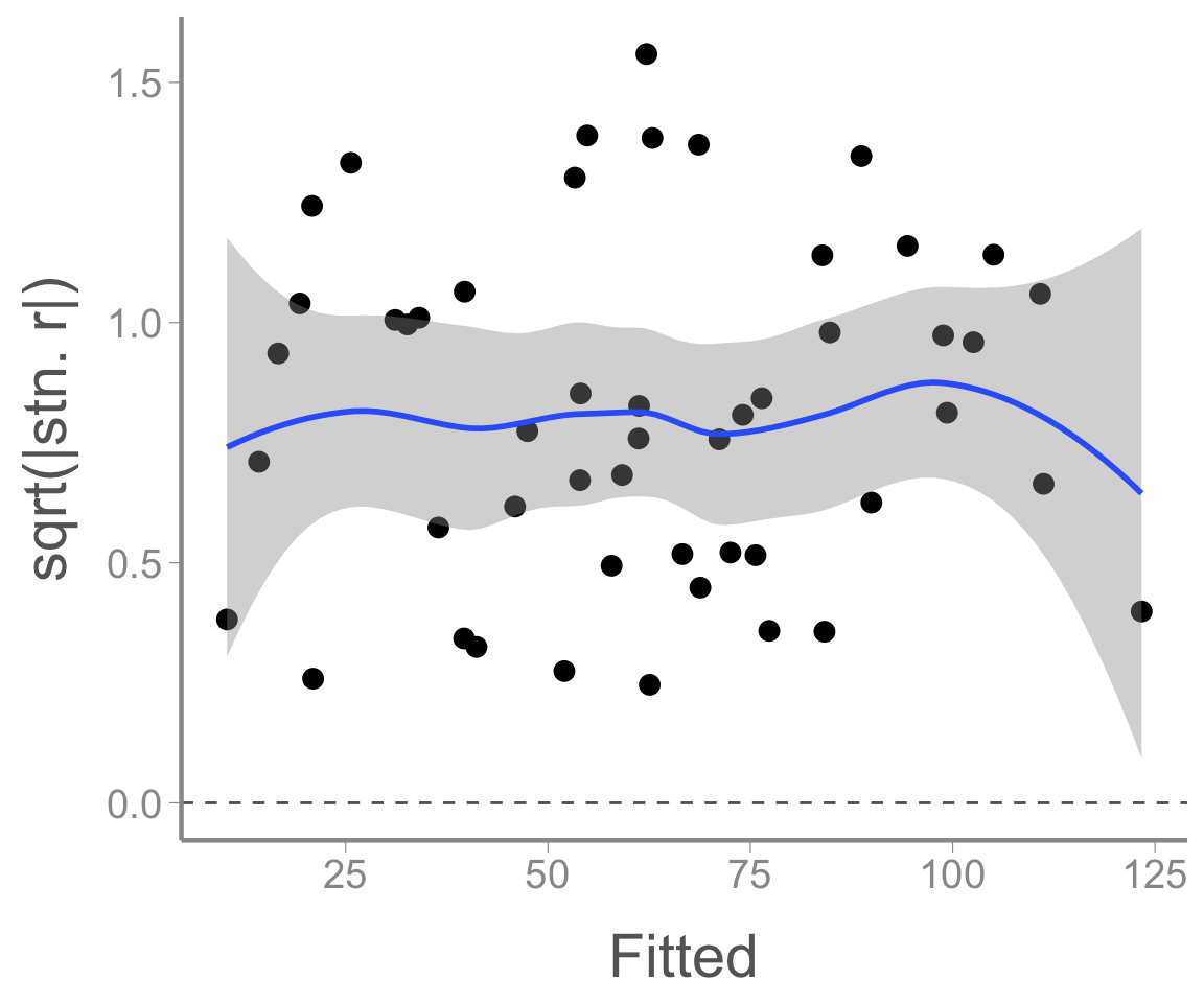
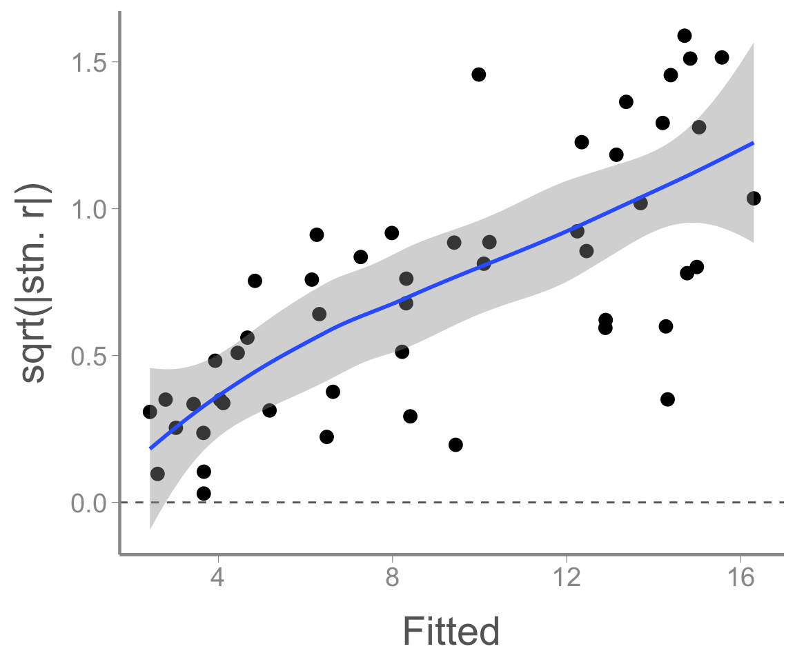
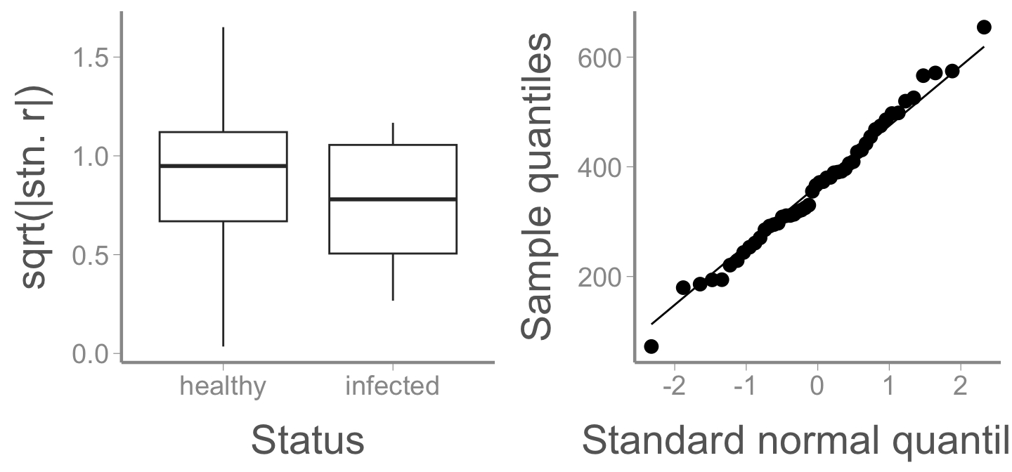
Heteroscedasticity can also be assessed by plotting the square root of residuals. Violations will appear as increasing or decreasing trends

Normality

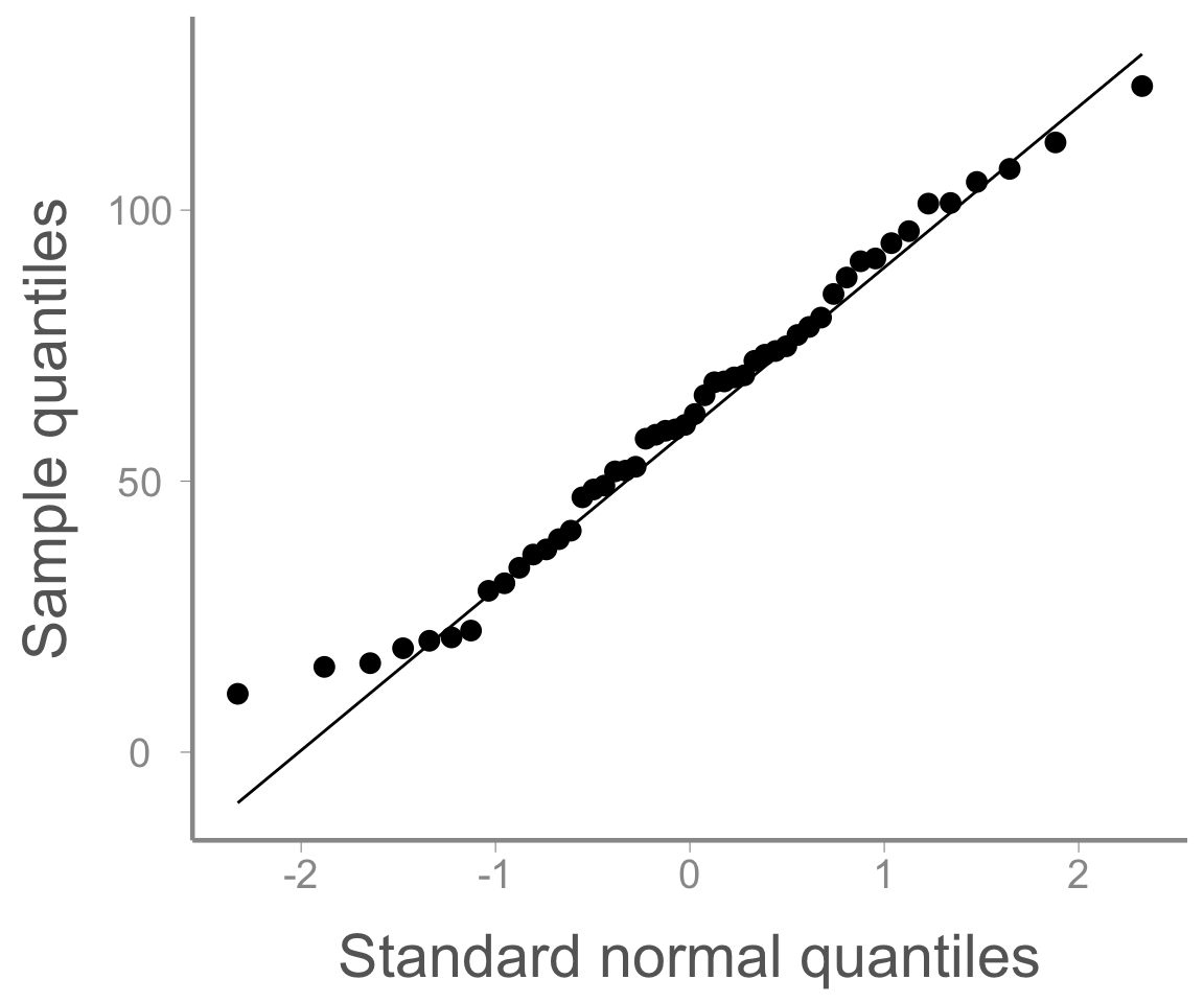
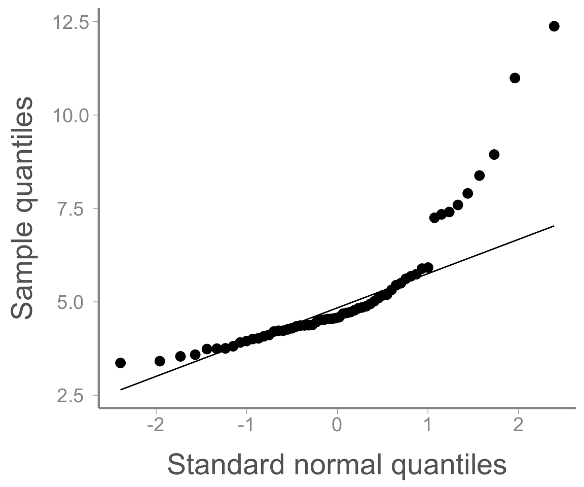
Normality is usually assessed using quantile-quantile (Q-Q) plots, which plots the observed quantiles of the residuals vs. the expected quantiles of normally distributed data

Large deviations from the line indicate deviations from normality

Evaluating models with factors

Because all of the models we have seen so far this semester are linear models, they all share the same assumptions

Testing assumptions of models with factors (t-test, ANOVA) is therefore no different than testing assumptions of models with continuous predictors

data("tunadata")
fm2 <- lm(growth ~ status, data = tunadata)

Null hypothesis testing

It is also possible to “test” whether assumptions are met:

check_normality(fm1)

OK: residuals appear as normally distributed (p = 0.377).

check_heteroscedasticity(fm1)

OK: Error variance appears to be homoscedastic (p = 0.957).

where the null hypothesis is that the data don’t violate the assumption being test (so \(p>0.05\) is good)

However, remember that the assumptions are about the population, not the sample

• samples can deviate from assumptions, even if they are met for the population

• deviations are more likely for small sample sizes

• there is always some judgement necessary when testing assumptions

We will explore some of these tests in lab

Independence

Non-independence of residuals is more difficult to test but is often related to un-modeled structure in the data

• points close in space/time tend to be more alike than distance points

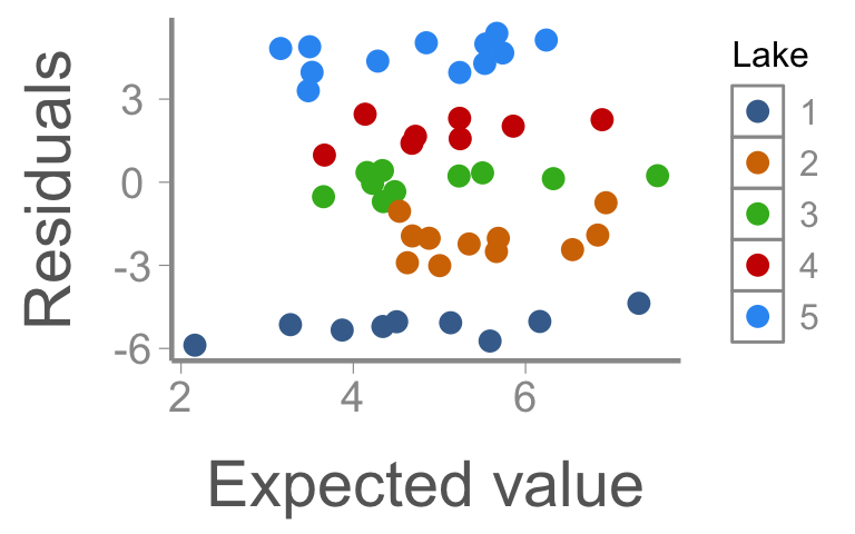
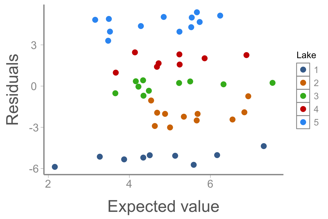
• observations within “groups” (e.g., study plots, growth chamber, lakes) tend to be more alike than individuals from other groups

Often, non-independence can be judged based on knowledge of the sampling design/system

• sometimes can be seen as “clustering” in residual plots

Independence

Sometimes, non-independence can be remedied by including relevant covariates in the model

• e.g. lm(y ~ x + Lake)

• we’ll learn more about this and related approaches in a few weeks

What happens when assumptions are violated?

One consequences of sampling is that our samples will likely depart from assumptions to some degree

So rather than asking:

“Do my data violate the assumptions of my model?”

It can be useful to ask:

“Do my data violate the assumptions of my model enough to change my conclusions?”

Fortunately, linear models are relatively robust to minor (or even moderate) departures from the assumptions

What happens when assumptions are violated?

General rules of thumb:

• Minor assumption violations will not generally bias estimates of \(\hat{\beta}_0\), \(\hat{\beta}_1\), etc.

• For large sample sizes, Central Limit Theorem often ensures that residuals of many types of data are normally distributed (or at least pretty close)

• Standard errors (and therefore confidence intervals, p-values, etc) will be biased when assumptions are violated

• In general, violating assumptions results in standard errors that are too small. What does this do to p-values?

Looking ahead

Next time: Principles of Causal Inference

Reading: Causal Inference in R, chp 3