LECTURE 14: causal inference in observational studies

Outline

1) Motivation

2) Examples

3) Visualizing confounders using DAGs

4) Controlling confounders using multiple regression

5) Other types of relationships and what to do with them

6) Minimal adjustment sets

Motivation

The flexibility of multiple regression models makes them powerful statistical tools but also raises an important question:

How do you know what predictors to include in your model?

• In experimental settings, the structure of multiple regression models is often determined by the experimental design

  • All treatments are included as predictors in the model

  • Interactions are included based on a priori hypotheses¹

  • Known sources of extraneous variation can be included to increase power

• In observational studies, it is is often less clear which combination(s) of predictors should be included in a model

  • It is increasingly common to have many predictors associated with each reponse

  • As the number of predictors grows, the number of potential combinations grows even faster

A few points

• Although deciding which predictors to include is really an issue of selecting among alternative models, this lecture is not about “model selection” in the conventional sense

• In fact, this lecture is not really about statistics at all. It is about using our scientific understanding to learn about cause and effect

• Warning: Some of the material in this lecture goes against conventional practices used in ecology/natural resources

  • Although causal inference is a well-developed field in its own right, these topics are not widely used in natural resources

  • In fact, many common practices you will encounter or be advised to use² actually conflict with best practices for causal inference

  • Often, there is no right or wrong “answer.” Using and defending your choices requires confidence and some degree of comfort with uncertainty

Example 1

• The Bleary Groundfinch is an imaginary bird species that is sexually-dimorphic (males are larger than females)

• During winter, both sexes defend individual territories that are mainly used for nocturnal roost sites

• The species roosts on the ground and it is thought that they compete for territories with dense shrub cover to minimize predation risk

• To determine whether shrub cover influences survival, researchers radio-tagged an equal number of male and female birds and then tracked them for several weeks, recording the fate (survived or died) of each bird

• They also located the nocturnal roost location of each individual and used vegetation surveys to quantify the average shrub density of each roost location

Question: Which covariates (cover, sex, or both) should the researchers include in their analysis? Why?

Example 1

Initially, the researchers fit two regression models³, one for each covariate

fit1 <- glm(survive ~ Sex, data = groundfinchdata, family = "binomial")
broom::tidy(fit1)

# A tibble: 2 × 5
  term        estimate std.error statistic  p.value
  <chr>          <dbl>     <dbl>     <dbl>    <dbl>
1 (Intercept)    1.10      0.333     3.30  0.000981
2 SexMale        0.217     0.476     0.456 0.648   

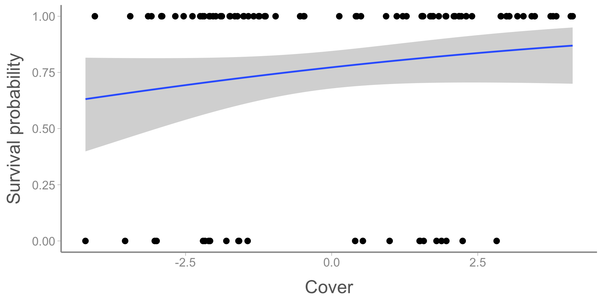
fit2 <- glm(survive ~ Cover, data = groundfinchdata, family = "binomial")
broom::tidy(fit2)

# A tibble: 2 × 5
  term        estimate std.error statistic     p.value
  <chr>          <dbl>     <dbl>     <dbl>       <dbl>
1 (Intercept)    1.22      0.243      5.04 0.000000473
2 Cover          0.163     0.108      1.51 0.131      

Example 1

Next, they fit a model with both covariates:

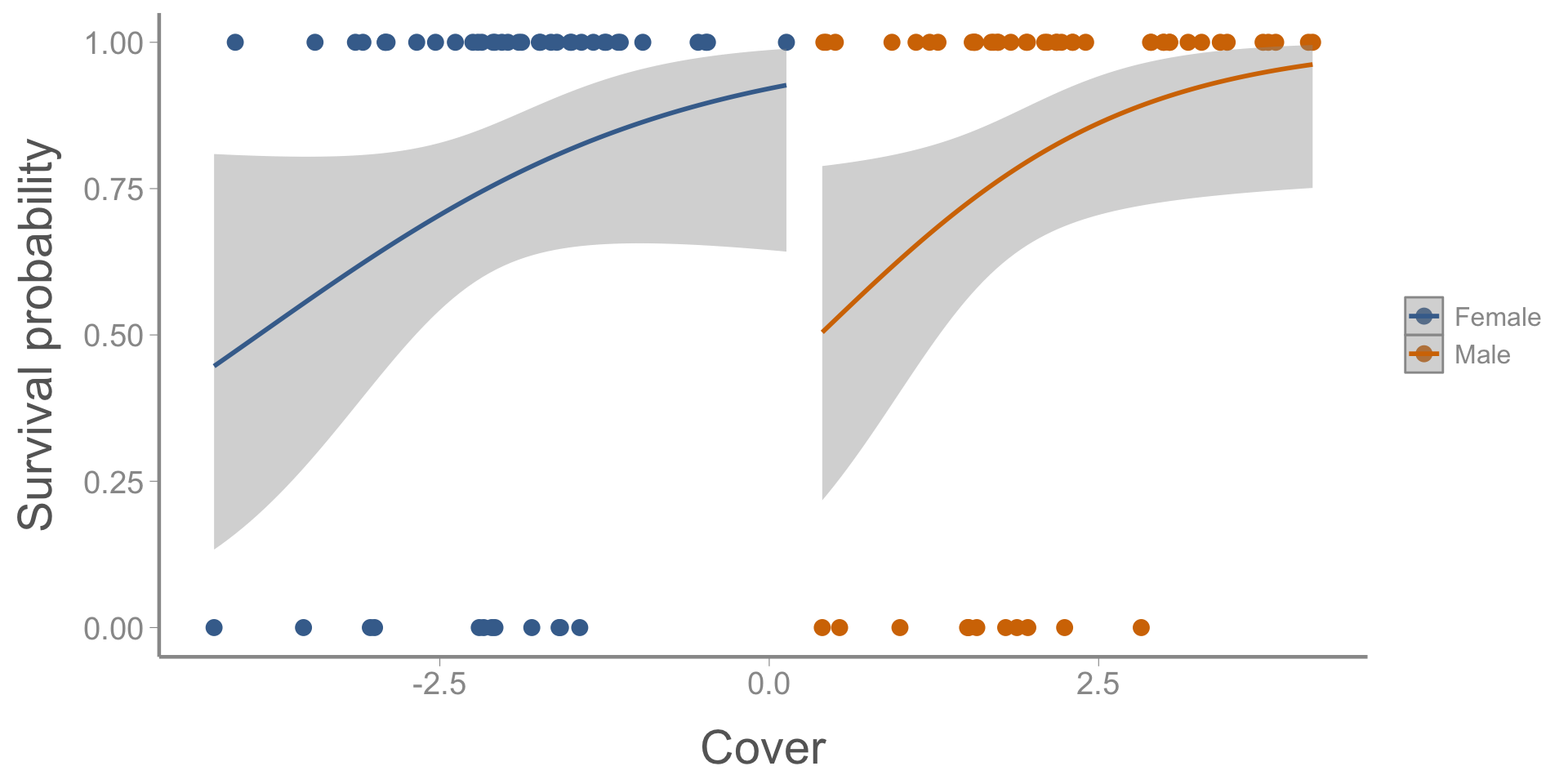
fit3 <- glm(survive ~ Sex + Cover, data = groundfinchdata, family = "binomial")
broom::tidy(fit3)

# A tibble: 3 × 5
  term        estimate std.error statistic  p.value
  <chr>          <dbl>     <dbl>     <dbl>    <dbl>
1 (Intercept)    2.70      0.740      3.65 0.000258
2 SexMale       -2.83      1.26      -2.24 0.0249  
3 Cover          0.744     0.287      2.59 0.00958 

Questions:

• What are your conclusions about the effect of sex and cover on survival?

• Why might the effect size (and sign) of sex have changed so dramatically when cover was added to the model?

Example 2

• A grad student is studying efforts to recover populations of the made-up, endangered Heirloom Trillium.

• The student is sent a dataset containing 20 years of surveys from a nature preserve containing a large population of the species.

• The data includes:

  • The number of plants at the end of summer (response variable)
  • The number of plants found at the beginning of the spring
  • An index of acorn mast the previous fall
  • The estimated number of deer within the study area

Question: Which covariates should the student include in their analysis? Why?

Example 2

The student initially notices that there is a strong negative association between abundance at the end of summer and acorn mast the preceding fall

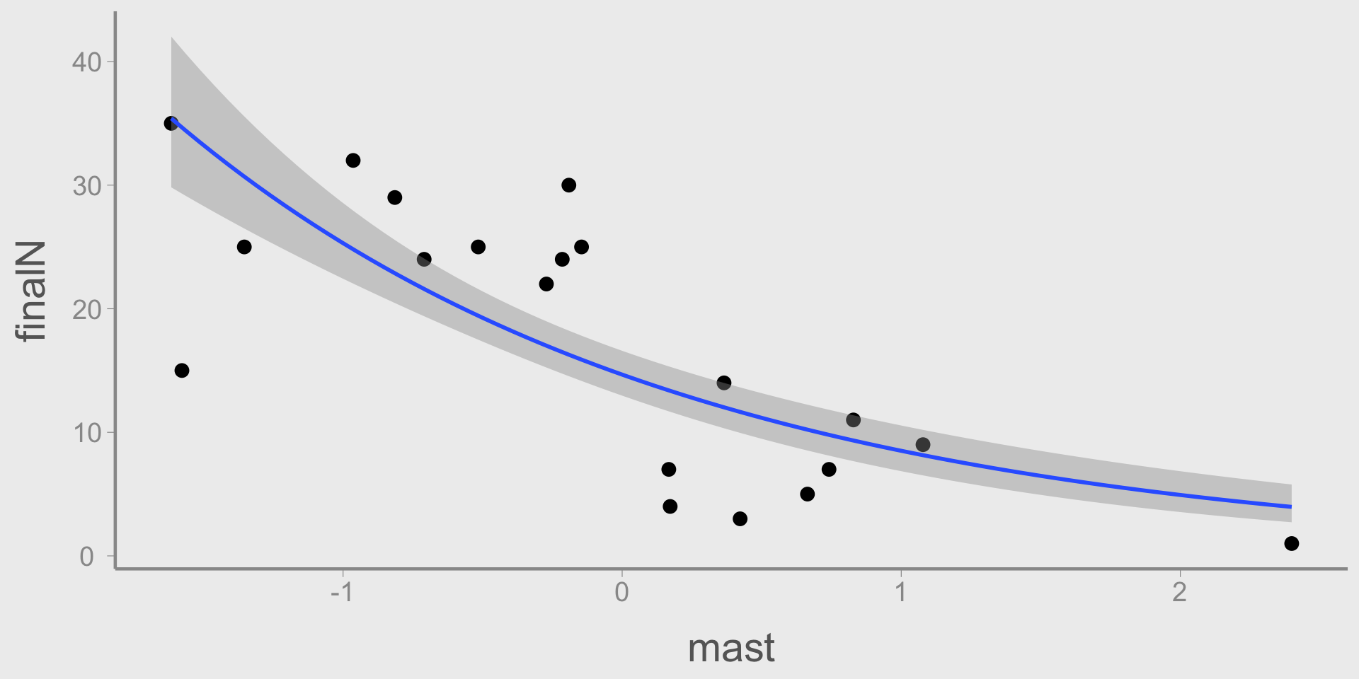
fit1 <- lm(finalN ~ mast, data = trilliumdata)
broom::tidy(fit1)

# A tibble: 2 × 5
  term        estimate std.error statistic       p.value
  <chr>          <dbl>     <dbl>     <dbl>         <dbl>
1 (Intercept)    16.7       1.63     10.2  0.00000000622
2 mast           -8.43      1.70     -4.96 0.000102     

Example 2

Nervous that his analysis was insufficient, the student decided to fit additional models to test whether other predictors may also influence Trillium abundance:

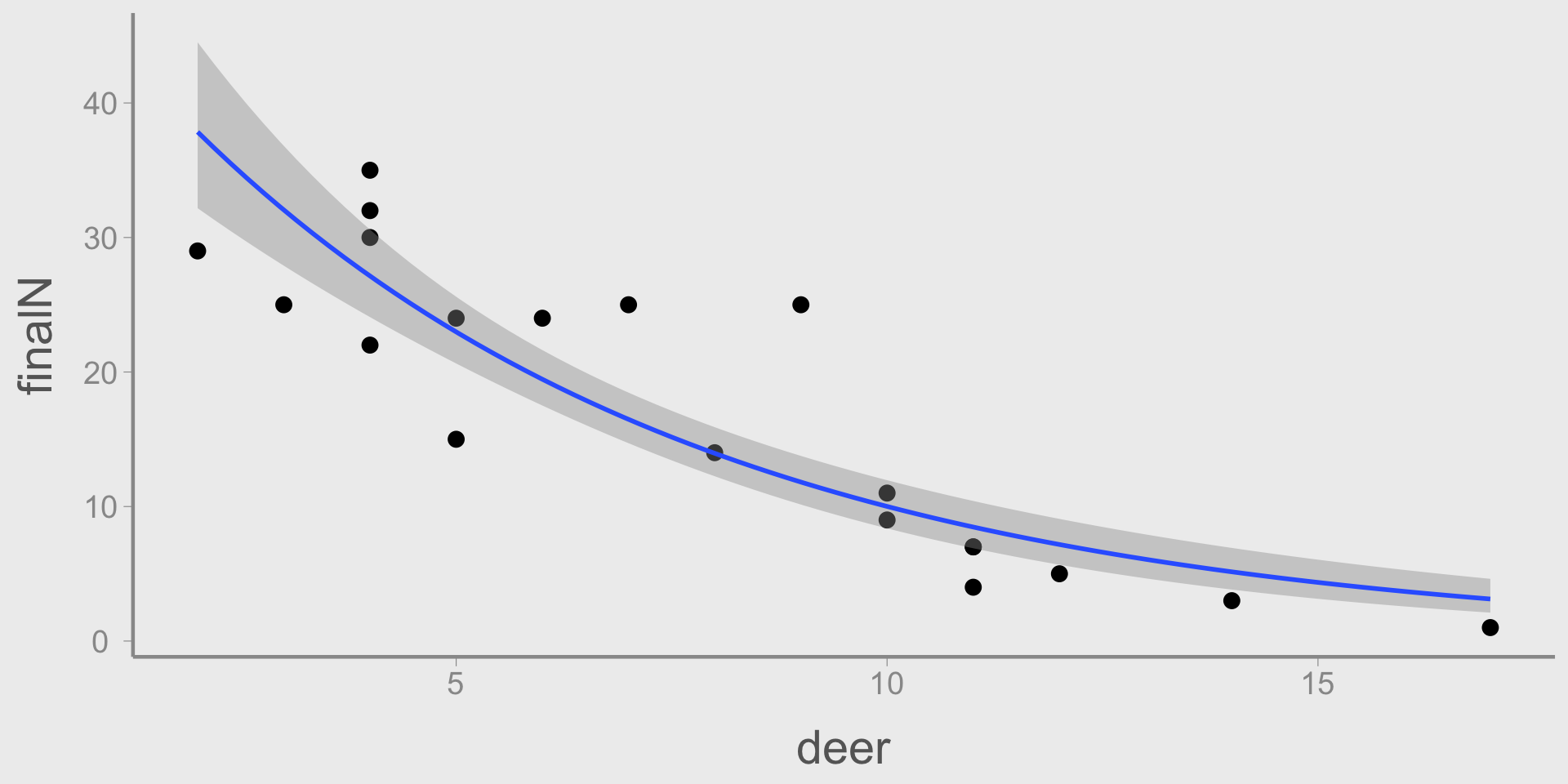
fit2 <- lm(finalN ~ mast + initN, data = trilliumdata)
broom::tidy(fit2)

# A tibble: 3 × 5
  term        estimate std.error statistic    p.value
  <chr>          <dbl>     <dbl>     <dbl>      <dbl>
1 (Intercept)   -12.5      6.26      -2.00 0.0613    
2 mast           -7.42     1.17      -6.37 0.00000701
3 initN           1.12     0.235      4.75 0.000186  

fit3 <- lm(finalN ~ mast + initN + deer, data = trilliumdata)
broom::tidy(fit3)

# A tibble: 4 × 5
  term        estimate std.error statistic     p.value
  <chr>          <dbl>     <dbl>     <dbl>       <dbl>
1 (Intercept)    5.73      3.94       1.45 0.165      
2 mast          -1.71      0.962     -1.78 0.0948     
3 initN          0.957     0.117      8.15 0.000000432
4 deer          -1.74      0.235     -7.39 0.00000152 

Questions:

• Why did the effect of mast change when deer abundance was added to the model?
• Is it reasonable to conclude that acorn mast affects Trillium abundance?

Example 3

• Researchers are studying the traits that influence “boldness” in fictitious Fruitcake Lizards

• The researchers searched for and captured lizards that they encountered, then used a well-established method to quantify the boldness of each individual

• The researchers used a linear model to quantify the relationship between body mass and boldness and found a strong negative association

• This result conflicts with previous studies of captive-reared Fruitcake Lizards that found no relationship between body size and boldness

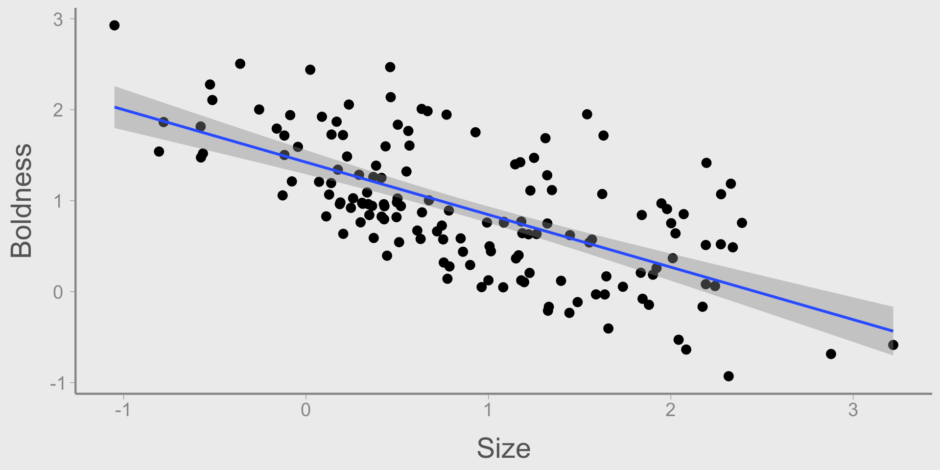
Question: Assuming that captive-rearing has no effect on boldness, why might the researchers have observed this strong, negative association?

Building multiple regression models

The previous examples, although somewhat simplified, illustrate a common scenario you will encounter: multiple models can be fit to the same data set and your conclusions depend on which model you choose

Conventional approaches to selecting among models are based on associations among predictor variables (e.g., strong correlations) and/or some type of model selection procedure (e.g., AIC)

• As with any statistical procedure, these approaches base modeling decisions on the strength of statistical associations

  • “Causal salad”

• However, we should base these decisions on our understanding of why variables are associated with each other

Causal inference

In lecture 7, we learned that: Correlation = Causation + Confounding + Noise

Manipulative experiments remove the effects of confounding by randomizing treatments or holding confounding sources of variation constant

In observational studies, we can’t randomize our “treatment” variables, which often results in non-exchangeable groups

• So does that mean we can’t remove the effects of confounders? Not necessarily

Another example: A common question in life history studies is whether there is a trade off (i.e., negative relationship) between reproduction and survival. Researchers monitor the annual reproductive effort and subsequent survival of wild coyotes and find that, in contrast to their predictions, individuals that raised more offspring had higher survival than individuals that raised fewer offspring

We can’t conclude that higher reproductive effort causes higher survival because coyotes with different reproductive success are unlikely to be exchangeable. Why?

Visualizing your hypotheses

When thinking about sources of variation, it can be helpful to visualize hypothesized relationships among variables

• Simple graphical models with nodes (variables) and edges (arrows pointing from cause to effect) are often useful for this goal

In the coyote example, we might hypothesize the following:

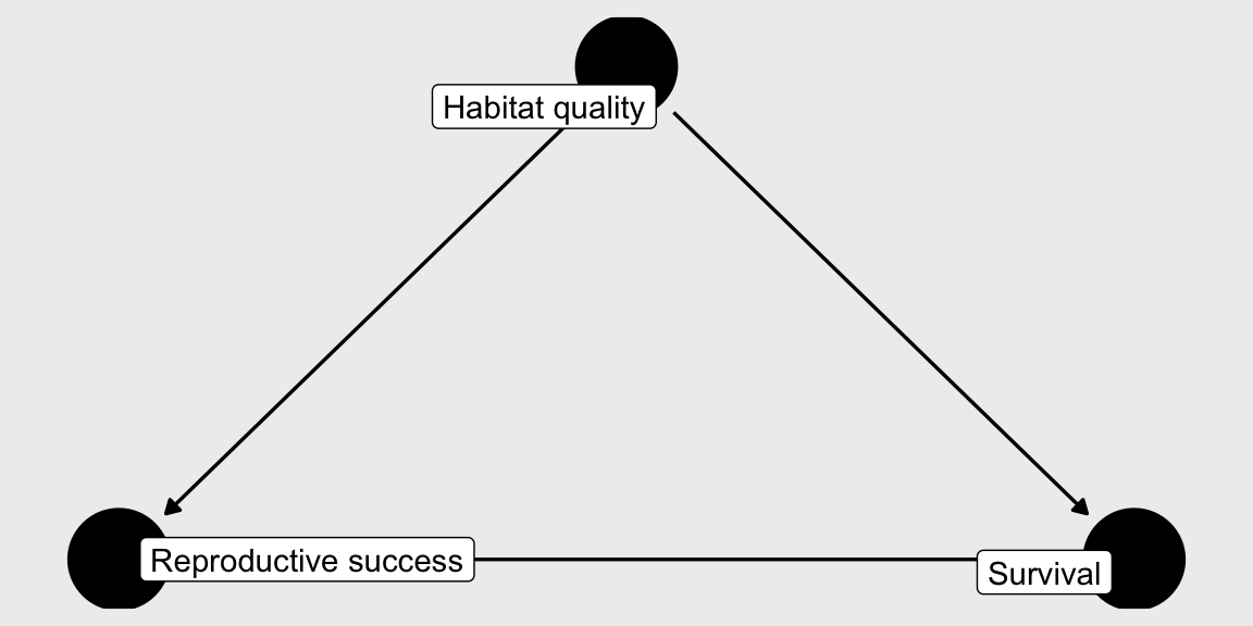
Visualizing your hypotheses

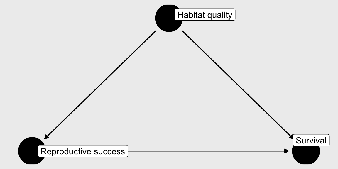
• This type of graphical model is referred to as a directed acyclical graph (DAG)

• DAGs are central to many causal inference methods

Building DAGs

DAGs are graphical models that describe causal relationships between variables

The purpose of a DAG is to articulate the direction of causal effects that influence both the response variable and covariates

All DAGs must be:

• Directed: \(X \longleftrightarrow Y\) is not possible

• Acyclic: \(X \longrightarrow Y \longrightarrow Z \longrightarrow X\) is not possible⁴

DAGs:

• Do not encode anything about the form of relationships (e.g., direction, non-linearity, interactions, etc.)

• Should include all important variables⁵, regardless of whether you have data on them or not!

Using a DAG for causal inference

The benefit of DAGs is that they allow us to identify variables that could prevent conclusions about whether \(X\) causes \(Y\)

• As we’ve already seen, one type of variable DAGs help us identify are confounders

• Confounders open backdoor paths that can create statistical associations between \(X\) and \(Y\), even when no causal effect exists⁶

• In manipulative experiments, randomization removes the association between \(Z\) and \(X\) (i.e., closes the backdoor path)⁷

• How do we remove the effect of confounders in observational studies?

  • Multiple regression!⁸

  • Multiple regression can accomplish statistically what experiments handle using design/randomization

Using multiple regression to remove confounding

Remember from lecture 12 how to interpret the slope parameters from multiple regression models:

The effect of \(X\) while holding all other variables constant

Sound familiar?

If \(Z\) is a confounder, multiple regression “removes” the effect of \(Z\) when measuring the effect of a treatment \(X\)⁹

So a DAG tells us which variables act as confounders and therefore which variables need to be included in our model

Example 1

Let’s use a DAG to figure out what might be happening in example 1. What is the relationship between predation risk, cover, and sex?

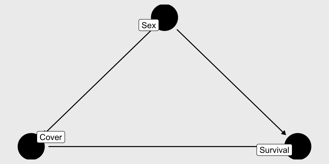
• From this DAG, it is clear that sex is a confounder of both cover and survival.

• Because it is a confounder, we have to control for it to quantify the causal effect of cover on survival¹⁰

  • What is the interpretation of the cover variable from the multiple regression model?

• We can also conclude that the model that includes only cover is the wrong model for our question. No model selection necessary!

Multicolinearity

Multicolinearity

One of the most commonly used justifications for excluding covariates from a model is multicolinearity, which is often defined as predictor variables that are strongly correlated with each other¹¹

Typical advice is to remove covariates that have strong, pairwise correlations (e.g., > 0.7)

But this is not good advice:

• Including correlated predictors does not violate any assumptions of linear models

• The purpose of multiple regression is to measure the effect of one predictor while holding others constant

• Often, omitting correlated variables is a bigger problem than including them

• As we have seen, confounding variables will almost always be correlated with \(X\) but should be included to control for their influence

Sometimes you should include correlated predictors

Pairwise correlations may indicate you should include a predictor:¹²

• In the life history trade-off example, habitat quality is likely to be strongly correlated with reproductive success

• Does this mean we can’t include habitat quality in the model? No! We need to include it if we want to isolate the effect of reproductive success

• With both parameters in the model, the coefficient associated with reproductive success tells us “after controlling for the effects of habitat quality, do coyotes with higher reproductive success have lower survival”

Sometimes you should include correlated predictors

Pairwise correlations may indicate you need to include a predictor:

• Researchers are interested in the effects of traffic on coyote movement. Exploratory analysis reveals that GPS-collared coyotes are more active during times of high traffic. Can we conclude that traffic increases movement? What might be confounding traffic?

• Time of day! Coyotes are crepuscular so they tend to move more in the morning and evening, when traffic is also highest (\(traffic \longleftarrow TOD \longrightarrow movement\))

• We need to include time of day if we want to isolate the effect of traffic

• With both parameters in the model, the coefficient associated with traffic tells us “after controlling for the effects of time of day, do coyotes move less when traffic is high”

  • As long as time of day and traffic are not perfectly correlated (traffic varies from day to day, especially weekends/holidays) and we have enough data, the regression model can disentangle their effects

Effects of multicolinearity

The previous examples hopefully clarify that including or removing predictors based solely on pairwise correlations is bad advice

But including highly correlated predictors is not without consequences:

• When variables are highly correlated, they contain little unique information about their individual effects

  • Statistically, perfectly correlated predictors are actually a single variable

• The higher the correlation, the higher the uncertainty associated with each predictor (indicated by large standard errors)

• The higher the correlation, the larger sample size needed to maintain statistical power

  • Disentangling the effects of highly correlated predictors is essentially a sample size issue, not a violation of model assumptions

When is multicolinearity a problem?

One instance that highlights when multicolinearity can be problematic¹³ is when covariates represent percentages that must sum to 1:

• Land use (% forest, % developed, % agriculture, etc.)

• Diet (% fruit, % insects, % seeds)

• Behavior (% of time foraging, % resting, % moving)

These covariates are structurally colinear - if you know the values of all but one category, you know the value of the last category

• If you change value of one category, value of other categories must also change

  • “What is the effect of \(X\) while holding all other parameters constant” is an impossible question to answer

• If you try to include every category as a predictor, many models with fail (error message or infinite standard errors)

  • Removing one (or more) categories may be necessary to fit the model

Multicolinearity - practical advice

• If covariates are correlated because of confounding, you need to include the confounder (if your goal is causal inference)

• If covariates are correlated because they essentially measure the same thing, you should remove all but one

• If covariates have a structural correlation (e.g., sum to 1), generally best to drop one category

• When you include correlated predictor variables, be prepared for larger standard errors (because that’s what is supposed to happen!)

• If standard errors are so big that they essentially render parameter estimates useless, you may need to simplify the model by removing covariates (but be sure you understand how that changes your interpretation!)

• Prediction is not effected by multicolinearity. If your goal is to predict, focus on predictive accuracy and don’t worry about pairwise correlations among covariates

other types of associations

Confounders are only one type of causal relationship. Several others are important to know about:

• Mediators

• Colliders

• Competing exposures

As with confounders, DAGs are a critical tool for understanding and identifying each of these types of relationships

Mediators

Mediators are variables that exist along a path between \(X\) and \(Y\)

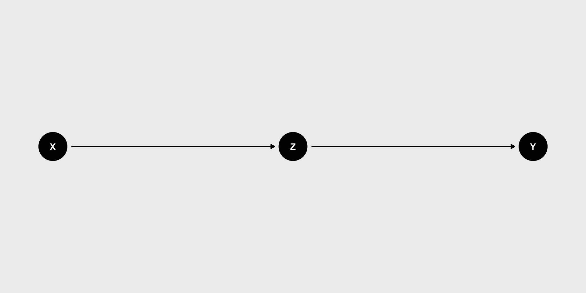
In a DAG, mediators have arrows pointing from \(X\) and to \(Y\)

• Often, mediators are the mechanism that causes \(X\) to influence \(Y\)

• If \(Z\) is a mediator, including it in the model “blocks” the effect of \(X\)

  • What is the effect of \(X\) after accounting for \(Z\)? None, if \(X\) acts through it’s effect on \(Z\)

• Mediators can sometimes be included in models to test whether \(Z\) might be the mechanism

• Including a mediator also allows you to measure the effect of \(X\) that is not due to \(Z\)¹⁴

Colliders

Confounders are common causes of \(X\) and \(Y\). Colliders are common effects of \(X\) and \(Y\)

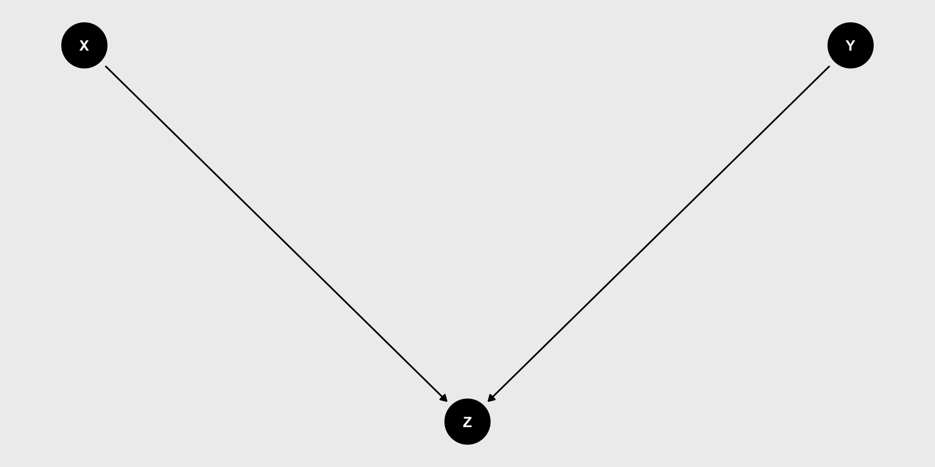
In a DAG, colliders have arrows pointing towards them from both \(X\) and \(Y\)

• Including colliders in models can cause associations between \(X\) and \(Y\) when none actually exists

• If you know there is a collider in your data, do not include it in your model

Colliders

Colliders are very common but understanding what they are and why the cause spurious relationships can be confusing¹⁵

A few examples:

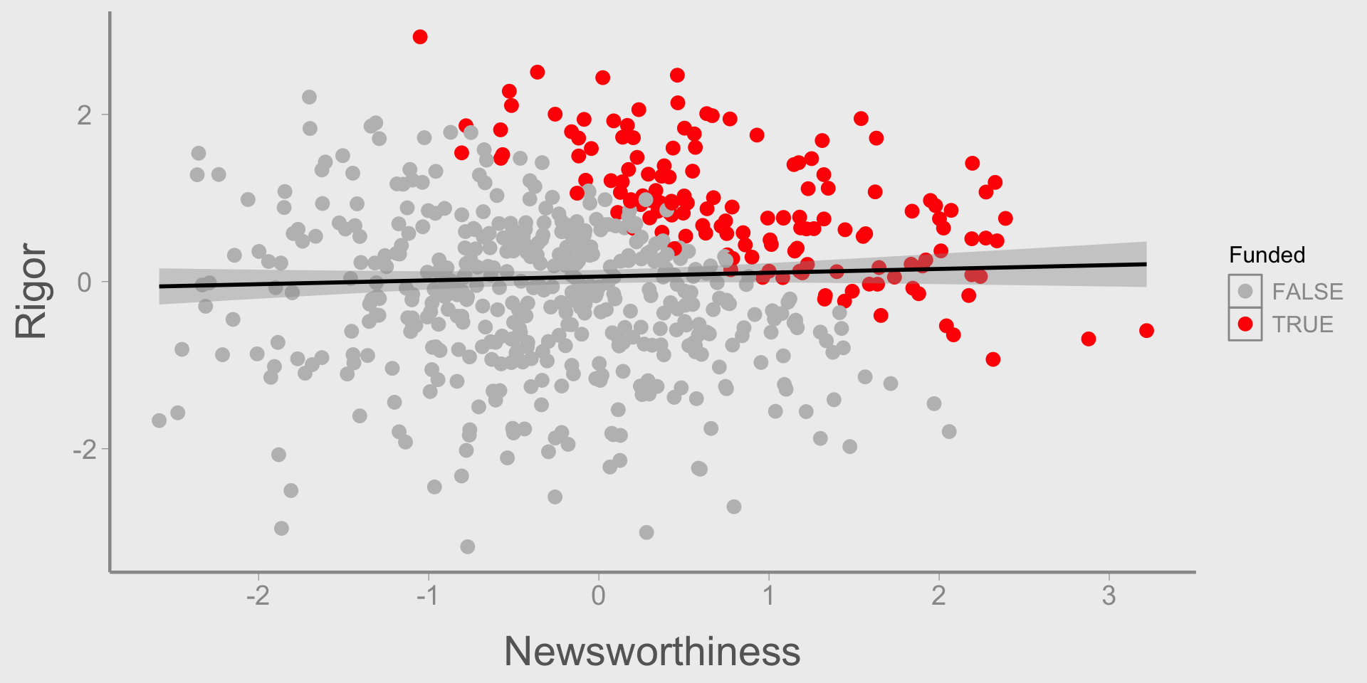
Research projects that get a lot of press are often low quality. Does rigor influence newsworthiness (or vice versa)?

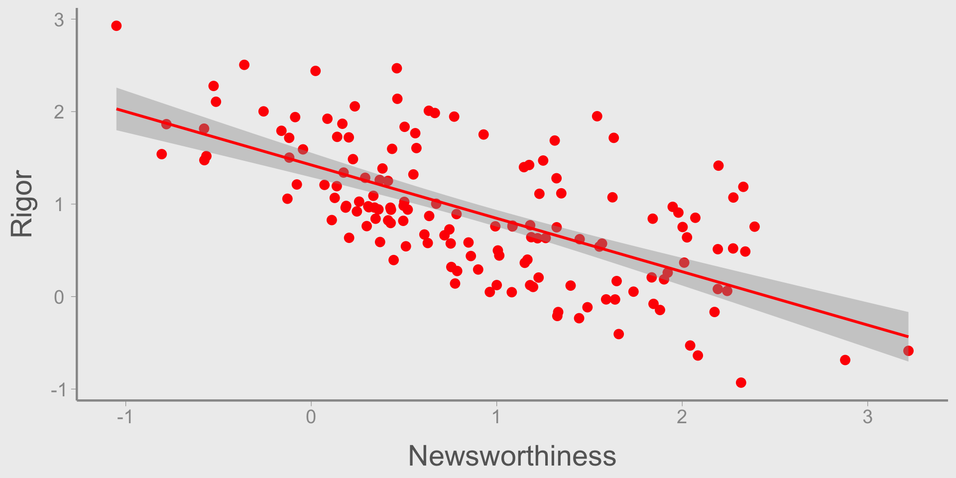
• To get funded, a proposal must either be very high quality or be very “newsworthy”

• Funding is a collider (quality \(\longrightarrow\) funding \(\longleftarrow\) newsworthy)

Colliders

Colliders are very common but understanding what they are and why the cause spurious relationships can be confusing¹⁶

A few examples:

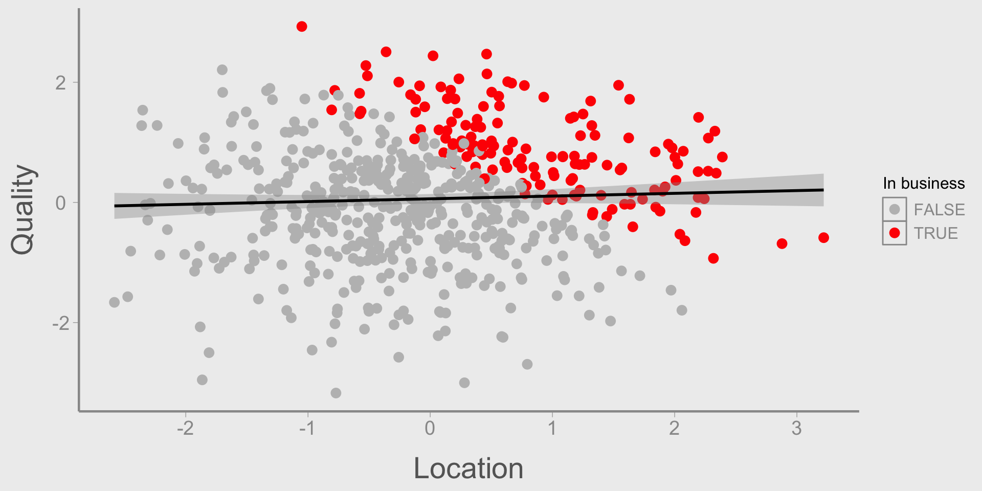
Restaurants in good locations tend to have worse food than restaurants in bad locations. Does location influence food quality?

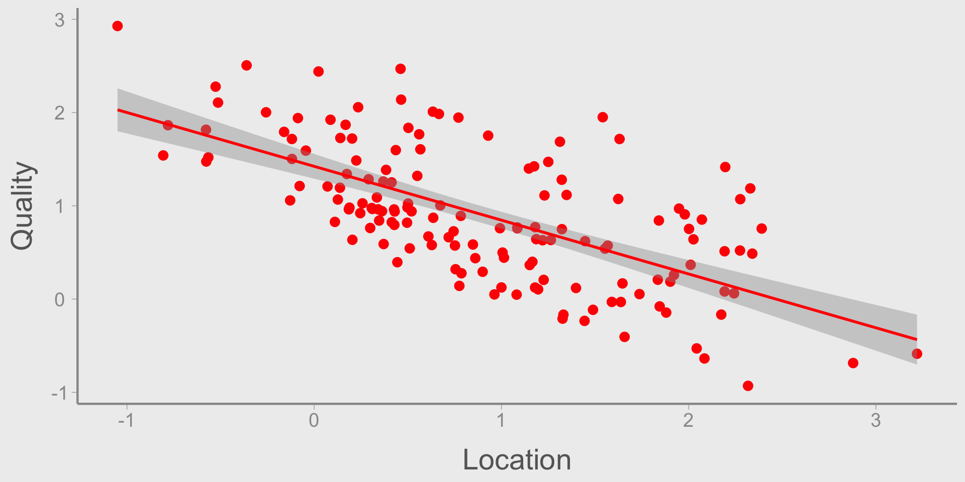
• Restaurants in bad locations have to be good to stay in business. Restaurants in good locations can get away with having lower quality food

• Staying in business is a collider (location \(\longrightarrow\) open \(\longleftarrow\) quality)

Colliders

Colliders are very common but understanding what they are and why the cause spurious relationships can be confusing¹⁷

A few examples:

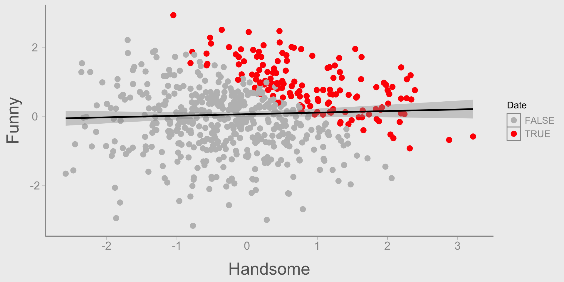
The guys your friend dates are either handsome or funny. Are good looks and sense of humor related?

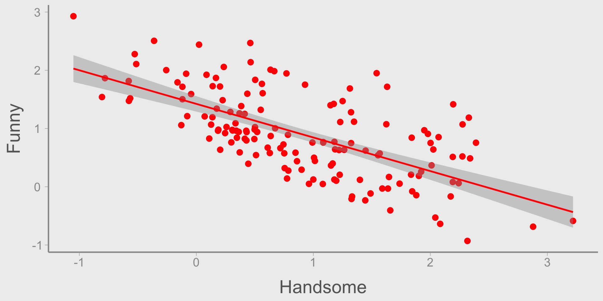
• Handsome guys can get a date even if they are boring. The rest of us have to be funny

• Getting a date is a collider (looks \(\longrightarrow\) date \(\longleftarrow\) humor)

Competing exposures

Competing exposures are variables that effect the response variable \(Y\) but are independent of the cause \(X\)

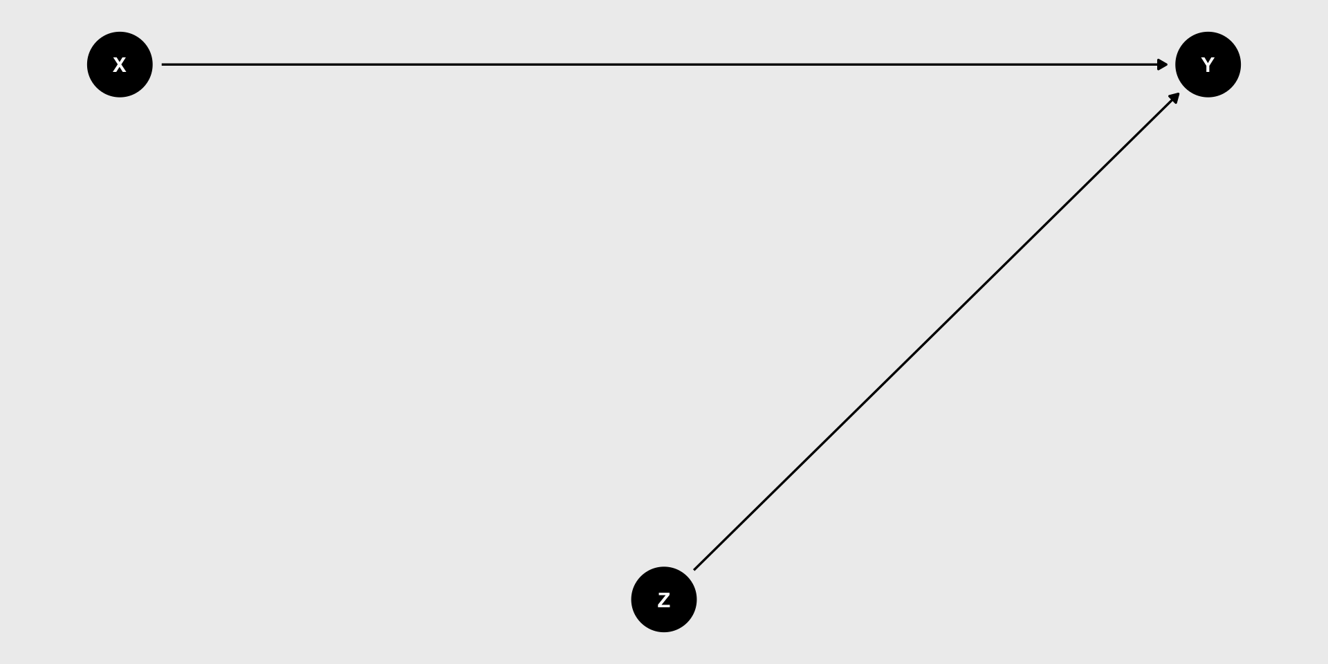
In a DAG, competing exposures have arrows pointing towards \(Y\) but not \(X\)

• Including competing exposures in models does not directly influence inference about the effect of \(X\) on \(Y\)

• Because competing exposures don’t influence causal inference about \(X\), choices about whether to include them in the model should be based on other considerations

  • Are they of interest?

  • Does including them provide more power for detecting the effect of \(X\)?

  • Does including them reduce precision of other model parameters?

Examples

Let’s return to the second and third examples from the beginning of lecture

• Why did the effect of mast change when deer abundance was included in the model? What is the relationship between fall acorn mast, deer abundance, and trillium counts?

• \(mast \longrightarrow deer \longrightarrow trillium\)

• Because deer is a mediator, including it in the model removes the effect of mast. But that does not mean mast is not a cause of Trillium abundance!¹⁸

• What is the role of initial abundance?

• \(mast \longrightarrow deer \longrightarrow trillium \longleftarrow abundance_{init}\)

• Because initial abundance is not a confounder or a mediator, including it in the model does not bias estimates of deer or mast. Why might you include it in the model?

Example 3

In laboratory studies, there was no effect of body size on boldness. So why did the researchers studying wild lizards find this relationship?

In the population, there is no link between boldness and body size

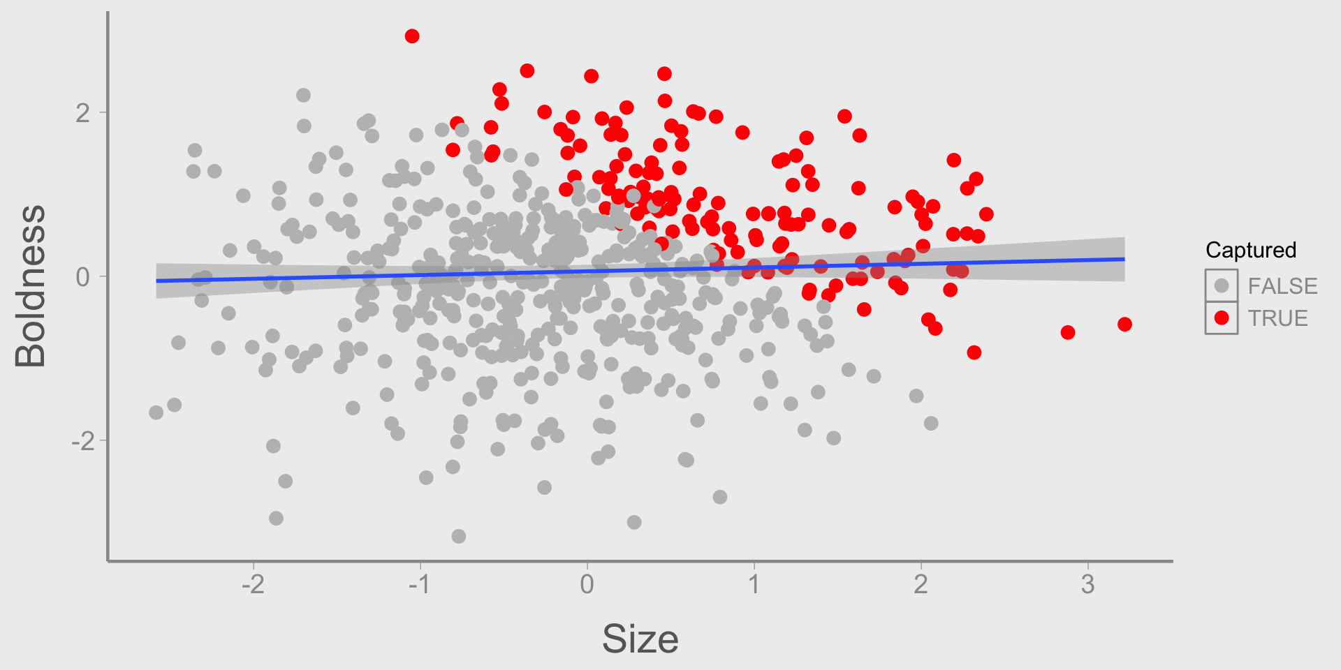
• Lizards only end up in the data set if they are captured

• Who gets captured? Lizards that are big or bold

• Who doesn’t get captured? Lizards that are small and shy

• In the observed sample, small lizards are almost guaranteed to be bolder than average¹⁹

Capture acted as a collider, which created a relationship where none actually existed.

Using DAGs

So far, we’ve used very simple graphs to show confounding caused by a single variable \(Z\).

However, confounding can often show up in more complex DAGs in ways that are not always quite so obvious.

Do you see any “open” paths from \(X\) to \(Y\) in the following graph?

• Paths are “open” if they are created by confounders/mediators; they are “closed” if they contain a collider

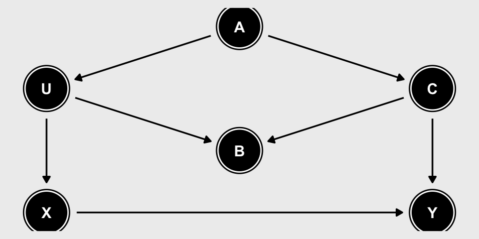
Open paths:

• \(X \longrightarrow Y\)

• \(X \longleftarrow U \longleftarrow A \longrightarrow C \longrightarrow Y\)

Why isn’t there an open path through \(B\)?

Using DAGs

Do you see any “open” paths from \(X\) to \(Y\) in the following graph?

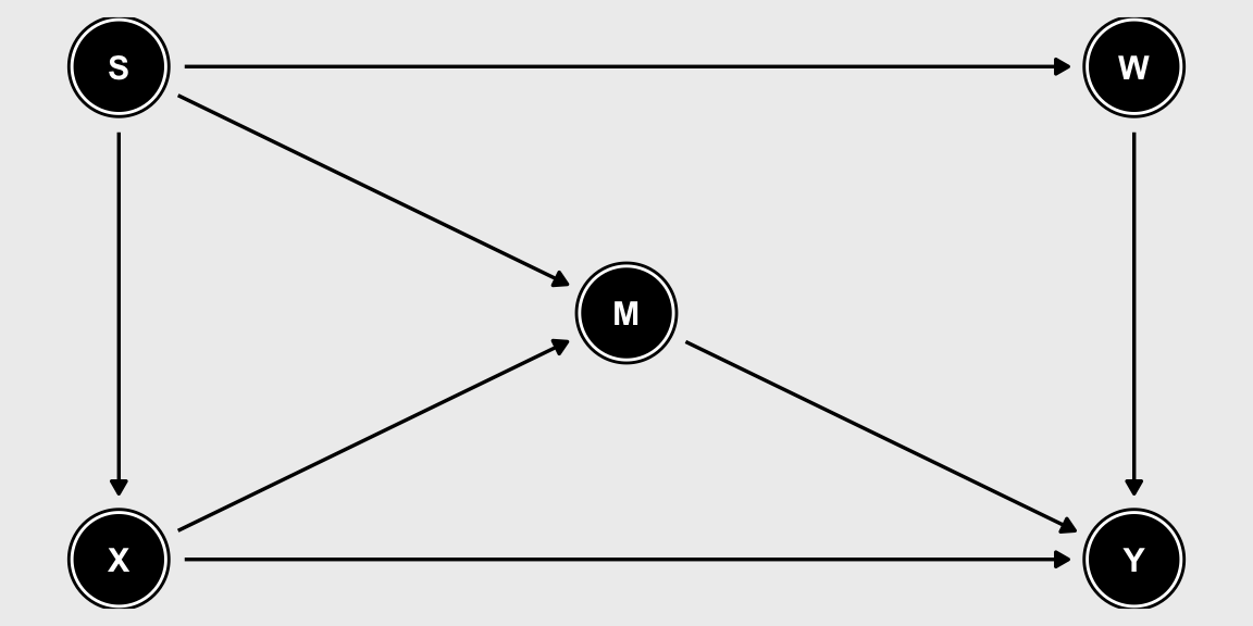
Open paths:

• \(X \longrightarrow Y\)

• \(X \longrightarrow M \longrightarrow Y\)

• \(X \longleftarrow S \longrightarrow M \longrightarrow Y\)

• \(X \longleftarrow S \longrightarrow W \longrightarrow Y\)

Using DAGs

Do you see any “open” paths from \(X\) to \(Y\) in the following graph?

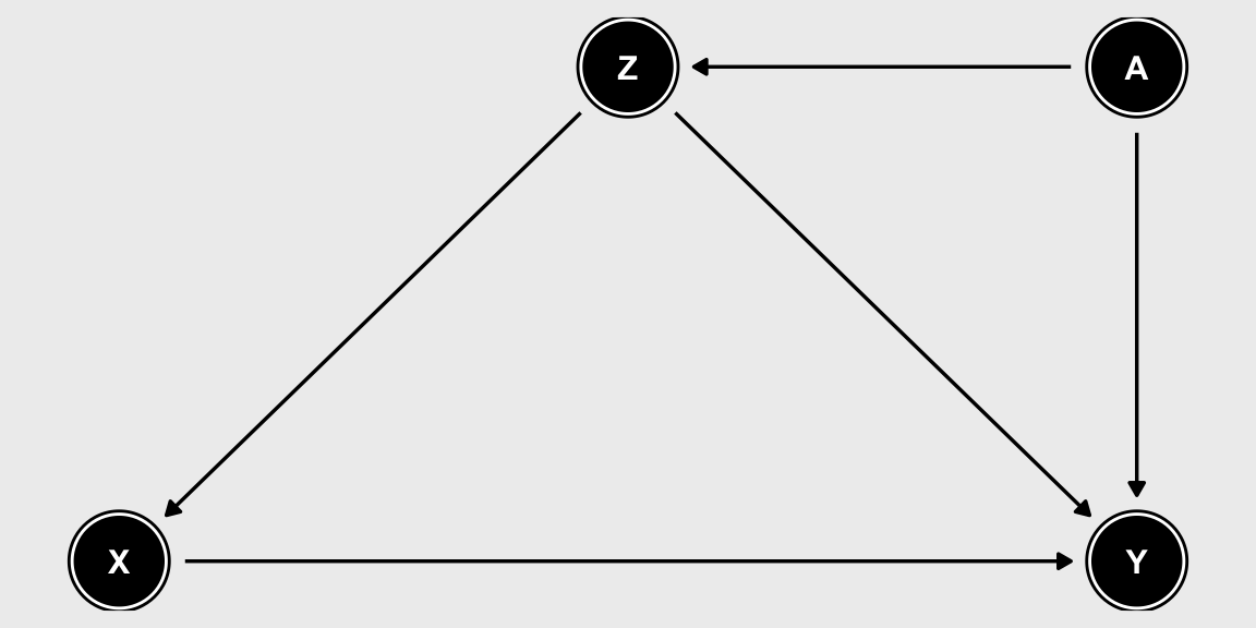
Open paths:

• \(X \longrightarrow Y\)

• \(X \longleftarrow Z \longrightarrow Y\)

• \(X \longleftarrow Z \longrightarrow A \longrightarrow Y\)

Minimal adjustment set

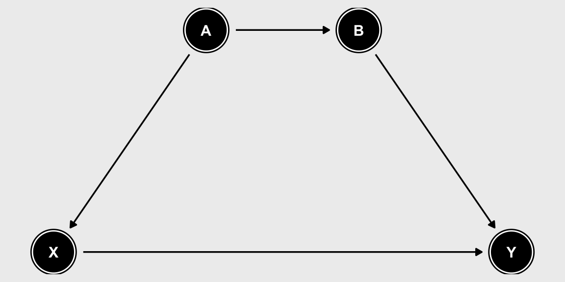
Conditioning on every variable along a confounding pathway is not necessary

Instead, we generally try to find the minimal adjustment set that blocks each confounding path

For example, in the following DAG we can condition on \(A\) or \(B\). We do not need to condition on both

Minimal adjustment set

What variables do we need to adjust in this example?

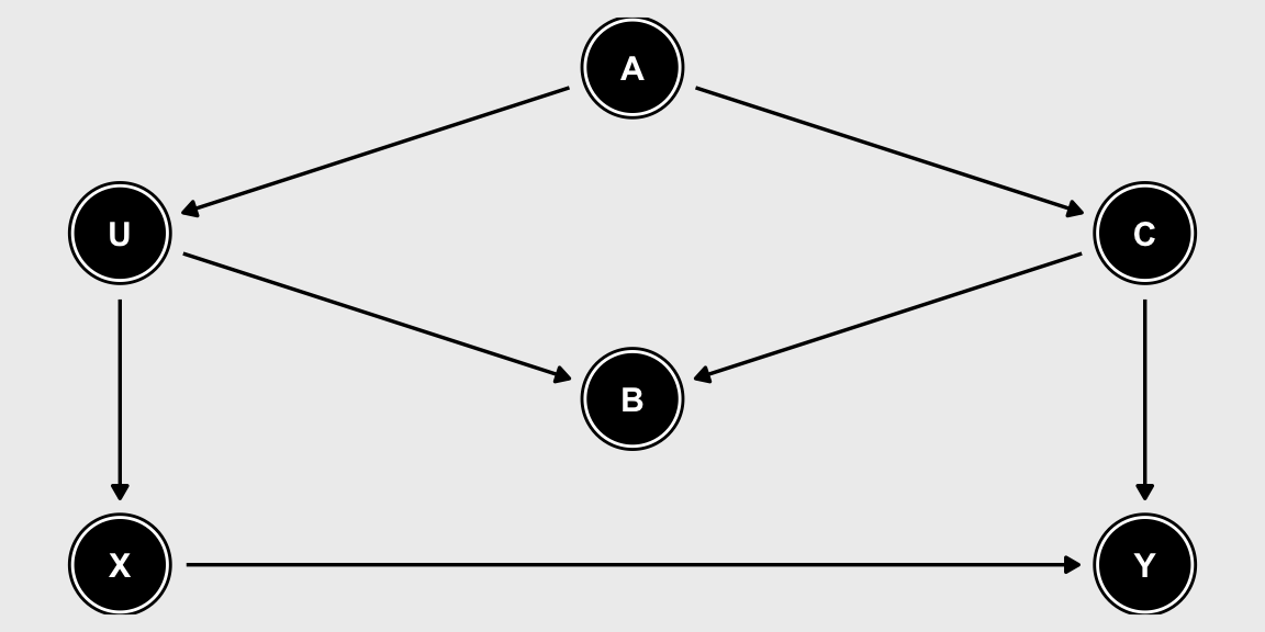
Which paths do we need to close?

• \(X \longrightarrow Y\)

• \(X \longleftarrow U \longleftarrow A \longrightarrow C \longrightarrow Y\)

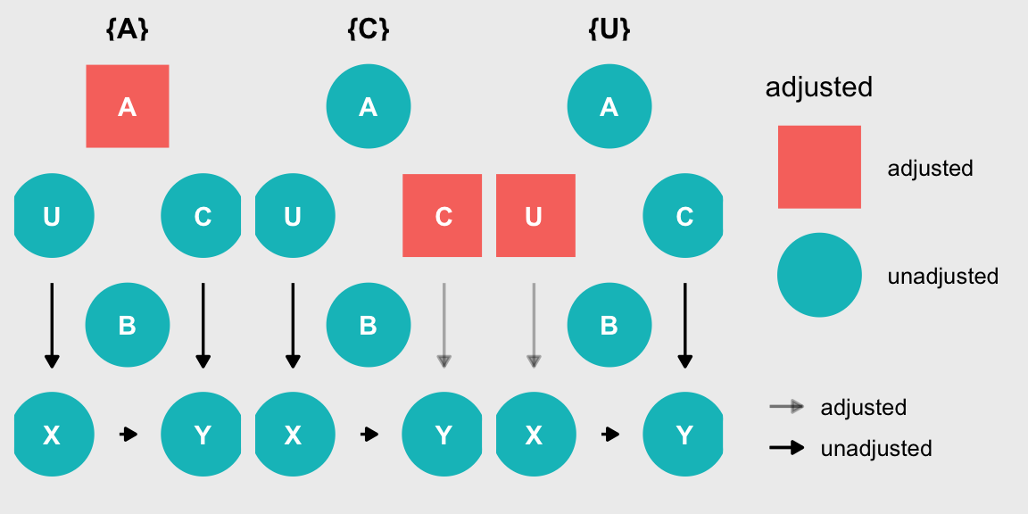
• To isolate the effect of \(X\), we can include \(A\) or \(C\) or \(U\)

• What happens if we include \(B\)?

Minimal adjustment set

What variables do we need to adjust in this example?

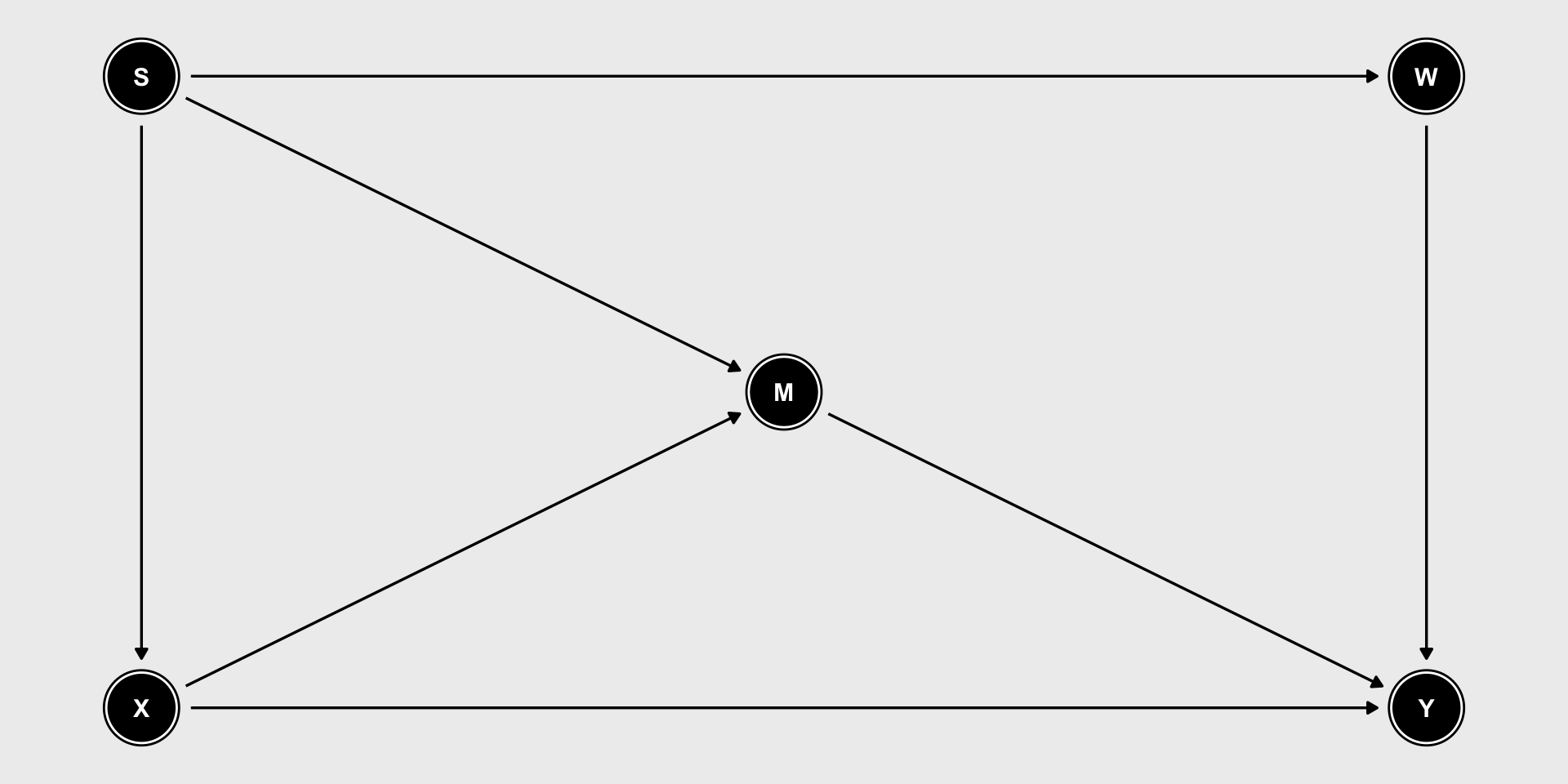
What paths do we need to close?

• \(X \longrightarrow M \longrightarrow Y\)

• \(X \longleftarrow S \longrightarrow M \longrightarrow Y\)

• \(X \longleftarrow S \longrightarrow W \longrightarrow Y\)

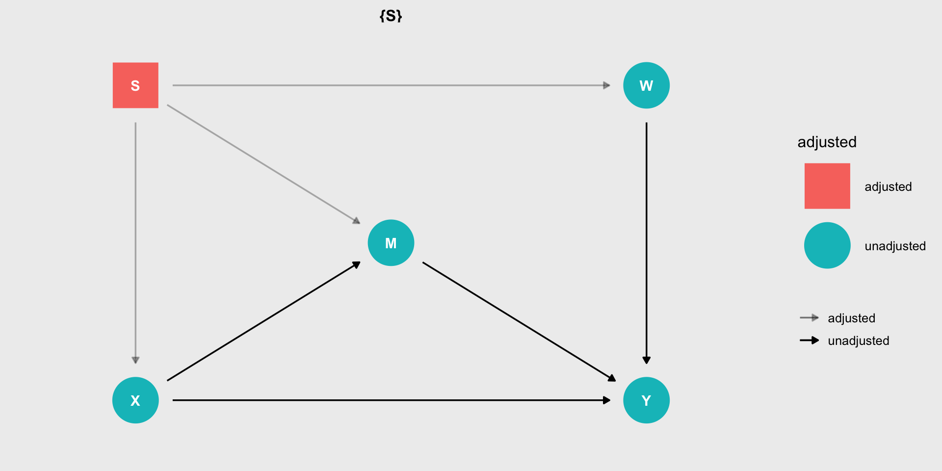
• To isolate the effect of \(X\), we only need to include \(S\)

• Why is including only \(W\) insufficient?

• What happens if we include \(M\)?

Minimal adjustment set

What variables do we need to adjust in this example?

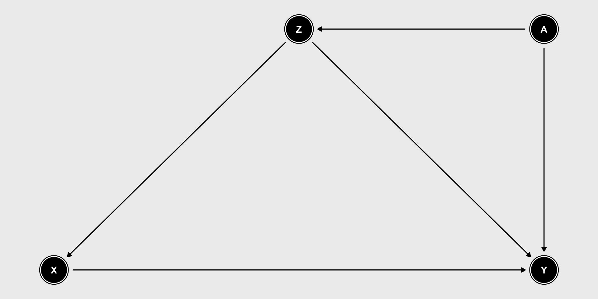
Open paths we need to close:

• \(X \longleftarrow Z \longrightarrow Y\)

• \(X \longleftarrow Z \longrightarrow A \longrightarrow Y\)

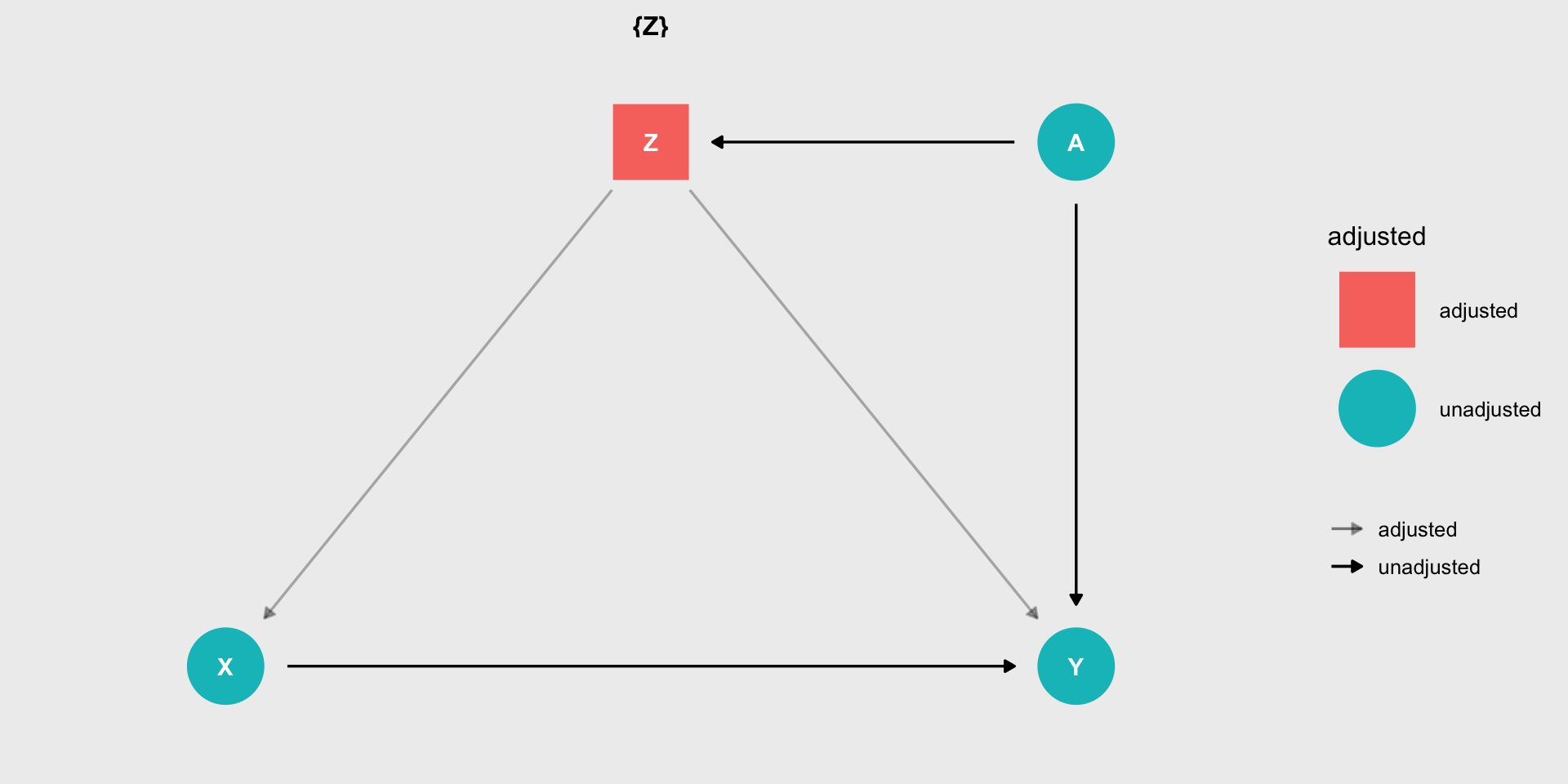
• To isolate the effect of \(X\), we only need to include \(Z\)

• Why is including only \(A\) insufficient?

More on DAGs

Building DAGs can be overwhelming due to the complexity of ecological systems

• Start with the response variable and think about variables that are likely to have meaningful effects

• Move to the main treatment variable(s) of interest. What variables likely influence it? How are those variables related to the response?

• If you were to conduct an experiment, which variables would you try to hold constant? What variables would you try to randomize over?

• Share your DAG with colleagues and explain your reasoning. Use feedback to revise the DAG until you are satisfied it captures the main variables influencing your system

• Remember that you should include variable whether you have data to measure them or not!

  • Better to know a confounder exists than to pretend it doesn’t

• Observed associations (or lack thereof) cannot tell you whether your DAG is correct. Building DAGs is a scentific exercise, not a statistical one

More on colliders

Colliders are often a form of “selection bias” - we only see data from observations that filter through some form of selection (e.g., capture, survival, self-reporting)

Part of what makes colliders challenging to identify is that they are often not variables we measure - There is not a column in the lizard data called “captured”

When colliders are not measured, they are essentially “in” the analysis by default

• DAGs can help identify potential colliders so that you can avoid being tricked by spurious associations

• More advanced modeling methods (e.g. hierarchical models) can sometimes be used to explicitly model the effects of colliders

When colliders are measured, they should not be included in the model

• Again, DAGs are the best tool for identifying colliders so you don’t accidentally create spurious relationships by adding them to the model

Summary

• Multiple regression is a powerful tool for causal inference in observational studies

• DAGs help guide model building by identifying confounders, mediators, and colliders

  • If your goal is to estimate causal effects of \(X\) on \(Y\), your regression model must include known confounders

  • Treat mediators with caution. Including mediators blocks paths between \(X\) and \(Y\), which will change results

  • Beware of colliders, they are often lurking behind the scenes and can cause spurious relationships

• Identifying confounders, mediators, and colliders is a scientific process.

  • Correlations, AIC, p-values cannot tell you whether your model is correct

• Also remember that the proper adjustment set for one variable may be different that the adjustment set for another variable

  • Identifying causal effects of different variables may require multiple models (Table 2 fallacy)

Additional resources

We have only scratched the surface regarding causal inference in observational studies.

There are many great resources for learning more about this topic, including:

• Dagitty: Web platform for constructing DAGs and identifying minimal adjustment sets

• Science Before Statistics: Recording of causal inference seminar by Richard McElreath (author of Stastistical Rethinking textbook)

• Causal Inference in R: Online text book about causal inference methods using R

• Byrnes, J.E. and Dee, L.E., 2025. Causal inference with observational data and unobserved confounding variables. Ecology Letters, 28(1), p.e70023.

Looking ahead

Next time: Model selection

Reading: Tredennick et al. (2021). A practical guide to selecting models for exploration, inference, and prediction in ecology Ecology 106(6): e03336 (posted on eLC)

Footnotes

1. Assuming adequate replication of all treatment combinations

2. including in previous versions of this course

3. specifically, they fit logistic regression models, which used for binary response data. We will learn more about logistic regression later in the semester but conclusions about the direction/significance of slope coefficients are the same as for linear regression

4. One common question when building DAGs in ecological settings is feedback loops. Don’t those create cyclic graphs? Often the answer is no, but only once we account for time. For example, density dependence may at first appear to be cyclic: \(N \longrightarrow \phi \longrightarrow N\), where \(N\) is population size and \(\phi\) is survival. But in reality, the graph is \(N_{t-1} \longrightarrow \phi_{t - 1} \longrightarrow N_t\), where \(t\) indexes year

5. Important is a vague term but generally a DAG should include any variables that could be biologically-relevant sources of variation

6. A common metaphor for DAGs is the flow of electricity. We want to know if electricity flows from \(X\) to \(Y\). Backdoor paths are those that allow electricity to flow into both \(X\) and \(Y\) from other variables

7. Closing the door is equivalent to blocking the flow of electricity

8. Multiple regression is not the only method to address confounding, but it is the only one we will cover in this class

9. This is what is meant by “conditioning on” or “controlling for” a variable

10. Assuming there are no other confounders

11. Though this is not quite the actual meaning

12. As we have discussed, variables can be correlated for many reasons. If the correlation is caused by confounding, then the confounder should be included in the model. But correlation does not automatically mean confounding, so again, identifying confounders depends on your scientific judgement

13. And helps explain what multicolinearity is

14. A model without mediator \(Z\) estimates the total effect of \(X\). A model that includes \(Z\) estimates the partial effect of \(X\). Both effects might be relevent depending on your question

15. Previously this semester we’ve used the term “spurious” to refer to associations that happen due to chance. If you collected a new sample, you probably wouldn’t find the association. But colliders do not produce random associations. If you repeat the study, you would still find the association. It’s a systematic effect of the collider

16. Previously this semester we’ve used the term “spurious” to refer to associations that happen due to chance. If you collected a new sample, you probably wouldn’t find the association. But colliders do not produce random associations. If you repeat the study, you would still find the association. It’s a systematic effect of the collider

17. Previously this semester we’ve used the term “spurious” to refer to associations that happen due to chance. If you collected a new sample, you probably wouldn’t find the association. But colliders do not produce random associations. If you repeat the study, you would still find the association. It’s a systematic effect of the collider

18. If you intervened by removing acorns, deer abundance would be lower, and Trillium abundance would be higher

19. Otherwise they wouldn’t be captured