In this activity, we will use the process of simulating data to understand what random effects are and how they are interpreted in hierarchical models.

Objectives

Simulate data sets with both fixed and random effect structure
Fit fixed and random effects models in JAGS

For this lab, let’s assume we’re interested in modeling the the body mass (g) of lizards as a function of body length (mm). We capture lizards on \(J\) study plots and measure the mass and length of each individual.

The model

In this example, we have a single continuous predictor variable and \(J\) levels of a factor. We’ll assume for now that the residual body mass of each individual is normally distributed after accounting for body length. This suggests that following model:

\[y_{ij} = \alpha_{[j]} + \beta \times x_i + \epsilon_i\]

\[\alpha_{[j]} \sim normal(\mu_{alpha}, \tau_{alpha})\]

\[\epsilon_i \sim normal(0, \tau)\]

First, set up the simulation parameters:

J <- 20               # Number of sites
N <- 200              # Number of observations
Length <- rnorm(N)    # Scaled body length

## Randomly determine each individuals study plot
plot <- sample(x = 1:J, size = N, replace = TRUE)
table(plot)

plot	Freq
1	8
2	8
3	14
4	6
5	15
6	8
7	10
8	4
9	12
10	5
11	15
12	16
13	14
14	6
15	8
16	16
17	11
18	7
19	4
20	13

Now, let’s set the parameters in the model:

mu.alpha <- 23   # Overall mean body mass
sigma.alpha <- 2 # standard deviation of group-level means
tau.alpha <- 1/sigma.alpha^2

alpha <- rnorm(J, mu.alpha, sigma.alpha)

beta <- 6     # Slope of body length on mass
sigma <- 3    # Residual standard deviation
tau <- 1/sigma^2

To create the linear predictor, we’ll use the model.matrix() function to create the model matrix corresponding to our model and then multiply it by our parameters:

Xmat <- model.matrix(~as.factor(plot) + Length - 1)
Xmat[1:5,c(1,2,3,21)]
#>   as.factor(plot)1 as.factor(plot)2 as.factor(plot)3  Length
#> 1                0                0                0  2.3513
#> 2                0                0                0  0.9134
#> 3                0                0                0 -0.8348
#> 4                0                0                0  0.6705
#> 5                0                0                0 -0.3413

Now use matrix multiplication to create the linear predictor:

linear.pred <- Xmat %*% c(alpha, beta)
head(linear.pred)
#>    [,1]
#> 1 37.88
#> 2 27.42
#> 3 19.79
#> 4 30.21
#> 5 24.14
#> 6 26.67

And finally generate the observations and combine the relevant vectors within a single data frame:

mass <- rnorm(N, mean = linear.pred, sd = sigma)
mass_df <- data.frame(plot = as.factor(plot), length = Length, pred_length = linear.pred, mass = mass)

ggplot(mass_df, aes(x = length, y = mass, color = plot)) +
  geom_abline(intercept = alpha, slope = beta) +
  geom_point() +
  scale_color_brewer() +
  guides(color = "none")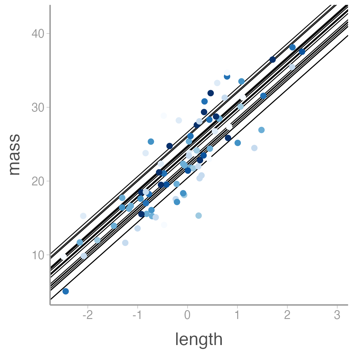

Fitting the model

Now we’re ready to fit the model in JAGS. Code for this model can be accessed with:

model.file <- system.file("jags/random_ancova.jags", package = "WILD6900")

Next, prepare the data, initial values, and MCMC settings. Notice the need to generate \(J\) starting values of \(\alpha\):

jags_data <- list(y = mass_df$mass, N = nrow(mass_df), 
                  J = J,
                  plot = plot,
                  x = mass_df$length)

jags_inits <- function(){list(mu.alpha = rnorm(1),
                              sigma.alpha = runif(1),
                              alpha = rnorm(J), # Notice we need J initial values 
                              beta = rnorm(1),
                              tau = runif(1))}

params <- c("mu.alpha", "sigma.alpha", "alpha", "beta", "tau", "sigma")

re_fit <- jagsUI::jags(data = jags_data, inits = jags_inits,
                    parameters.to.save = params, 
                    model.file = model.file,
                    n.chains = 3, n.iter = 10000, n.burnin = 2500, n.thin = 1)

print(re_fit)

	mean	sd	2.5%	25%	50%	75%	97.5%	Rhat	n.eff	f
mu.alpha	23.409	0.4215	22.546	23.140	23.418	23.687	24.221	1.000	7606	1
sigma.alpha	1.498	0.3804	0.847	1.233	1.462	1.725	2.352	1.000	4049	1
alpha[1]	23.882	0.8994	22.131	23.281	23.869	24.477	25.683	1.001	3720	1
alpha[2]	25.174	0.9543	23.373	24.516	25.153	25.794	27.123	1.000	10289	1
alpha[3]	21.824	0.7743	20.273	21.309	21.833	22.355	23.322	1.000	22500	1
alpha[4]	21.828	1.0506	19.717	21.123	21.859	22.562	23.784	1.000	22500	1
alpha[5]	22.681	0.7331	21.235	22.191	22.683	23.183	24.098	1.000	13398	1
alpha[6]	22.921	0.9034	21.132	22.320	22.930	23.527	24.678	1.000	22500	1
alpha[7]	24.221	0.8419	22.600	23.649	24.212	24.784	25.924	1.000	22500	1
alpha[8]	22.890	1.1111	20.650	22.159	22.911	23.637	25.041	1.000	15306	1

Just for kicks, let’s fit the same data to a model that assumes fixed-effects on the \(\alpha\)’s:

model.file <- system.file("jags/fixed_ancova.jags", package = "WILD6900")

jags_inits <- function(){list(alpha = rnorm(J), # Notice we need J initial values 
                              beta = rnorm(1),
                              tau = runif(1))}

params <- c("alpha", "beta", "tau", "sigma")

fe_fit <- jagsUI::jags(data = jags_data, inits = jags_inits,
                    parameters.to.save = params, 
                    model.file = model.file,
                    n.chains = 3, n.iter = 10000, n.burnin = 2500, n.thin = 1)

print(fe_fit)

	mean	sd	2.5%	25%	50%	75%	97.5%	Rhat	n.eff	f
alpha[1]	23.89	1.1141	21.69	23.15	23.90	24.64	26.07	1	7390	1
alpha[2]	25.95	1.1243	23.73	25.20	25.94	26.70	28.17	1	18945	1
alpha[3]	21.07	0.8502	19.39	20.50	21.07	21.64	22.71	1	22500	1
alpha[4]	20.17	1.2946	17.62	19.30	20.18	21.04	22.71	1	6441	1
alpha[5]	22.28	0.8333	20.63	21.72	22.28	22.85	23.92	1	13812	1
alpha[6]	22.35	1.1203	20.16	21.60	22.35	23.12	24.52	1	22500	1
alpha[7]	24.36	1.0073	22.36	23.68	24.35	25.03	26.34	1	22500	1
alpha[8]	21.68	1.5775	18.61	20.62	21.67	22.75	24.77	1	22500	1
alpha[9]	24.48	0.9201	22.67	23.85	24.47	25.10	26.28	1	14495	1
alpha[10]	21.74	1.4307	18.92	20.78	21.75	22.71	24.55	1	21272	1

Finally, combine results from the two models to visualize differences in the \(\alpha\) estimates:


compare_mods <- data.frame(alpha_mean = c(re_fit$mean$alpha, fe_fit$mean$alpha),
                           CI_2.5 = c(re_fit$q2.5$alpha, fe_fit$q2.5$alpha),
                           CI_97.5 = c(re_fit$q97.5$alpha, fe_fit$q97.5$alpha), 
                           n = c(table(plot) - 0.15, table(plot) + 0.15),
                           model = rep(c("Random", "Fixed"), each = J))

ggplot(compare_mods, aes(x = alpha_mean, color = model, y = n)) + 
  geom_vline(xintercept = mu.alpha, color = "grey50", linetype = "longdash") +
  geom_vline(xintercept = re_fit$mean$mu.alpha, color = "#CD0200", alpha = 0.75) +
  geom_errorbarh(aes(xmin = CI_2.5, xmax = CI_97.5), height = 0) +
  geom_point(size = 4, color = "white") +
  geom_point() +
  scale_color_manual(values = c("#446E9B", "#D47500", "black")) +
  scale_x_continuous(expression(alpha)) +
  scale_y_continuous("Sample size")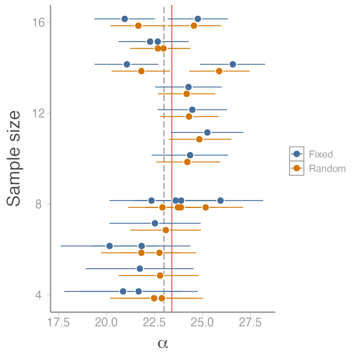

Quantifying changes in Coal tit (Periparus ater) abundance

In the remainder of this lab, you will use data from the Swiss Breeding Bird Survey to model changes in the abundance of Swiss Coal tits from 1999-2007.

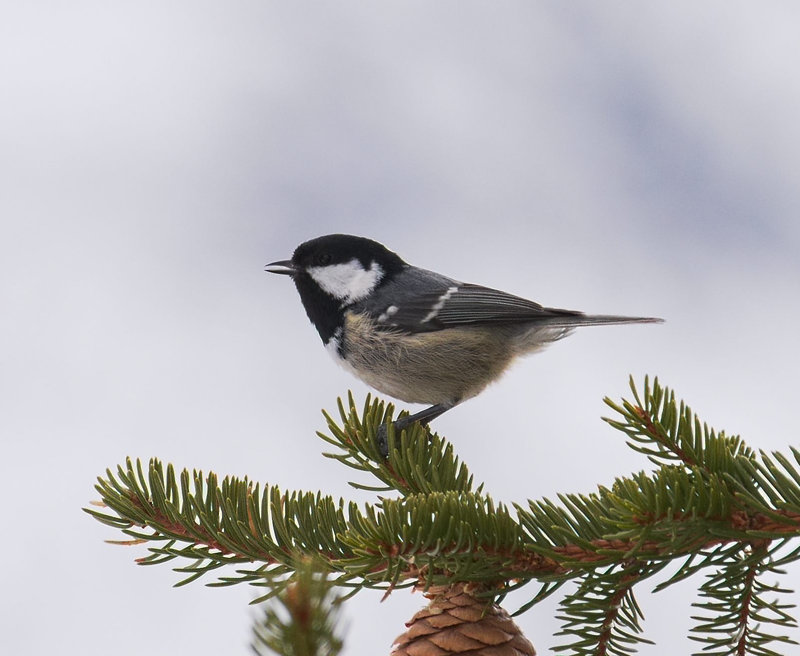
Photo by Andreas Eichler via WikiCommons

A data frame containing the counts and some additional information about each site (elevation and percent forest cover) and count (observer ID and whether it was an observers first time doing a BBS survey) is included in the WILD6900 package ¹:

data("tits")
head(tits)

site	spec	elevation	forest	y1999	y2000	y2001	y2002	y2003	y2004	y2005	y2006	y2007	obs1999	obs2000	obs2001	obs2002	obs2003	obs2004	obs2005	obs2006	obs2007	first1999	first2000	first2001	first2002	first2003	first2004	first2005	first2006	first2007
186	Coaltit	420	3	0	1	2	2	0	0	2	1	0	1576	1576	1576	1576	1576	1576	1576	1576	2125	1	0	0	0	0	0	0	0	1
NA.29	Coaltit	450	21	0	0	0	0	3	2	0	1	0	NA	NA	NA	NA	NA	NA	NA	NA	NA	NA	NA	NA	NA	NA	NA	NA	NA	NA
2.1	Coaltit	1050	32	NA	7	15	19	12	11	12	11	7	NA	2064	2064	2064	3299	3299	3299	3299	3299	NA	1	0	0	1	0	0	0	0
189.1	Coaltit	920	9	11	9	5	9	8	7	9	6	2	1576	2031	2031	2031	2031	2031	2031	2031	169	1	1	0	0	0	0	0	0	1
191.1	Coaltit	1110	35	27	24	21	19	22	31	28	9	18	1976	1976	1976	1976	1976	1976	1976	1976	1976	1	0	0	0	0	0	0	0	0
5	Coaltit	510	2	NA	0	2	1	0	0	0	0	0	NA	2158	3288	3288	3304	3304	3304	3304	3304	NA	1	1	0	1	0	0	0	0

Preparing the data

Before running any models, we will first prepare the data. JAGS will take the counts and predictor variables as matrices with dimensions of nSites x nYears. Those matrices can easily be created from the data frame:

C <- as.matrix(tits[5:13])
obs <- as.matrix(tits[14:22])
first <- as.matrix(tits[23:31])

matplot(1999:2007, t(C), type = "l", lty = 1, lwd = 2, main = "", las = 1, ylab = "Territory counts", xlab = "Year", ylim = c(0, 80), frame = FALSE)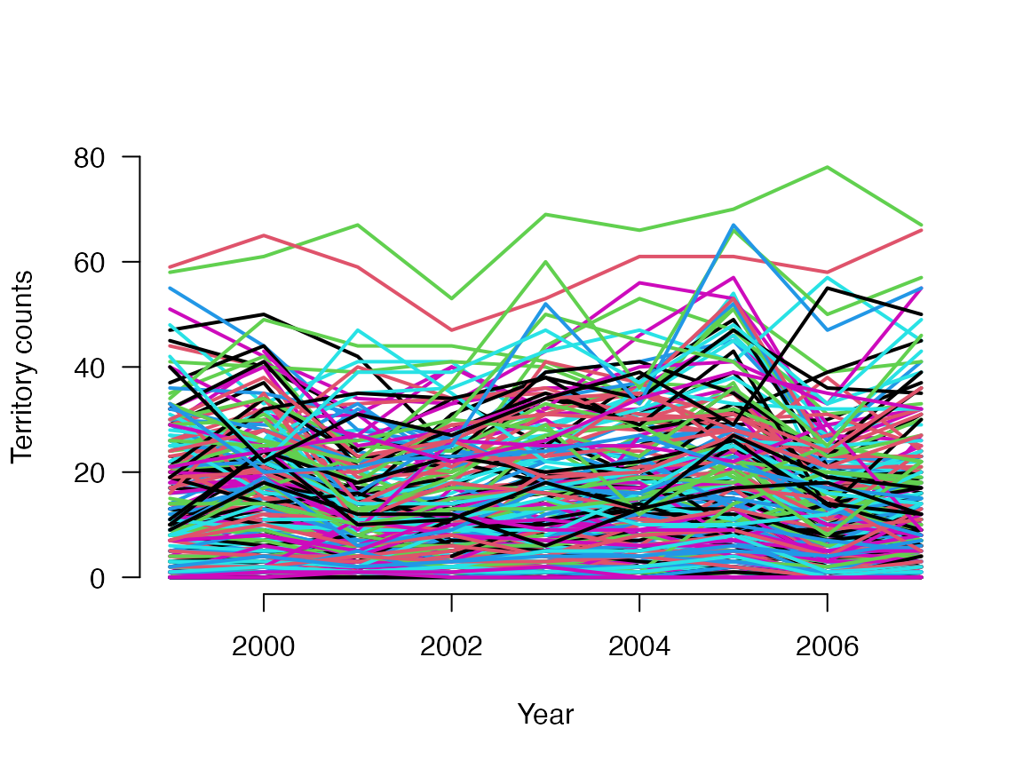

One issue with the obs and first matrices is that they contain NA values, which JAGS will not allow in predictor variables (they are ok in the response variable, as we will soon see). Some of the NA values correspond to years when a sites was not surveyed (in these cases, there will also be a NA in the C matrix). In addition, JAGS will want the observer ID as a continuous variable rather than a factor. We will first convert the obs levels into a numeric vector and the create a new matrix containing the correct numeric IDs:

a <- as.numeric(levels(factor(obs)))     # All the levels, numeric
newobs <- obs                            # Gets ObsID from 1:271
for (j in 1:length(a)){newobs[which(obs==a[j])] <- j }

Next, we need to fill in the NA values. For the observer ID, we’ll lump all missing values as a single value corresponding to the number of observers + 1. For the first matrix, we will code the NA values as 0, which corresponds to an ‘experienced’ observer. This will decrease our power to quantify the effect of being a novice observer but not to the extent that it will substantially alter our conclusions.

newobs[is.na(newobs)] <- length(a) + 1
first[is.na(first)] <- 0

The simplest count model

Let’s start by fitting the most simple model we can create for these data: the intercept-only model. In this model, we assume that the expected number of coal tits is constant, that is, it doesn’t vary across sites or years or observers.

On your own, write out the distribution, link function, and linear predictor for the intercept-only model. What parameters does this model include? What prior distribution(s) would be most appropriate for these parameters?

You can view the JAGS code for this model by running:

glm0_mod <- system.file("jags/GLM0.jags", package = "WILD6900")
file.show(glm0_mod)

Now prepare the data and MCMC settings to run this model:

# Bundle data
glm0_data <- list(C = t(C), nsite = nrow(C), nyear = ncol(C))

# Initial values
glm0_inits <- function() list(alpha = runif(1, -10, 10))

# Parameters monitored
params <- c("alpha")

# MCMC settings
ni <- 1200
nt <- 2
nb <- 200
nc <- 3

# Call JAGS from R
glm0 <- jagsUI::jags(data = glm0_data, inits =  glm0_inits,
                     parameters.to.save = params, 
                     model.file = glm0_mod, n.chains = nc, 
                     n.thin = nt, n.iter = ni, n.burnin = nb)

# Summarize posteriors
print(glm0, digits = 3)

# Check trace plots
jagsUI::traceplot(glm0)

Fixed site effects

The intercept-only model is obviously not a very good model of these counts but serves as a useful starting point for developing more complex models. As a start for building a better model, let’s add site as a fixed effect. In other words:

\[y_{ij} \sim Poisson(\lambda_j)\] \[log(\lambda_j) = \alpha_j\]

Modify the JAGS model from the previous example to run this fixed-site model. As a starting point:


sink("jags/GLM0.jags")
cat("
    model {

    # Prior
    alpha ~ dnorm(0, 0.01)    # log(mean count)

    # Likelihood
    for (i in 1:nyear){
    for (j in 1:nsite){
    C[i,j] ~ dpois(lambda[i,j])
    lambda[i,j] <- exp(log.lambda[i,j])
    log.lambda[i,j] <- alpha
    }  #j
    }  #i
    }
    ",fill = TRUE)
sink()

Be sure to change the name of the model file before running that code. Now modify the data and inits object as necessary to run the model in JAGS. Also note that in the jagsUI::jags() call you will need to reference the model file you just created rather than the model file from the previous example.

Additional complexity

Even with this relatively simple data set, you can create relatively complex models. On your own, try to fit the following models using the JAGS code from above as a starting point:

Fixed year and site effects
Random site effects
Random year effects
Random site and random year effects
Random site and random year effects and fixed first-year observer effect
Random site and random year effects, linear year effect and fixed first-year observer effect

One note about including multiple factors in the model. In the models with both site and year (as a factor), the model cannot estimate the predicted count for all combinations of both factors. Essentially, the model needs to set one level of one of the factors to a “reference” level to avoid over-parameterization. In JAGS, we have to do this manually by setting the prior for one level to zero:

eps[1] <- 0

Data and code from Kéry & Schaub 2015. Bayesian Population Analysis using WinBugs↩︎

Introduction to random effects and hierarchical models

WILD6900

2021-01-05