Lab 4: Completely randomized ANOVA
FANR 6750: Experimental Methods in Forestry and Natural Resources Research
Fall 2022
lab04_ANOVA.RmdBrief overview of ANOVA
ANOVA in R
Chainshaw data
The kick angle measurements for the 4 brands of chainsaw:
library(FANR6750)
data("sawData")

head(sawData)
#>    y Brand
#> 1 42     A
#> 2 17     A
#> 3 24     A
#> 4 39     A
#> 5 43     A
#> 6 28     B
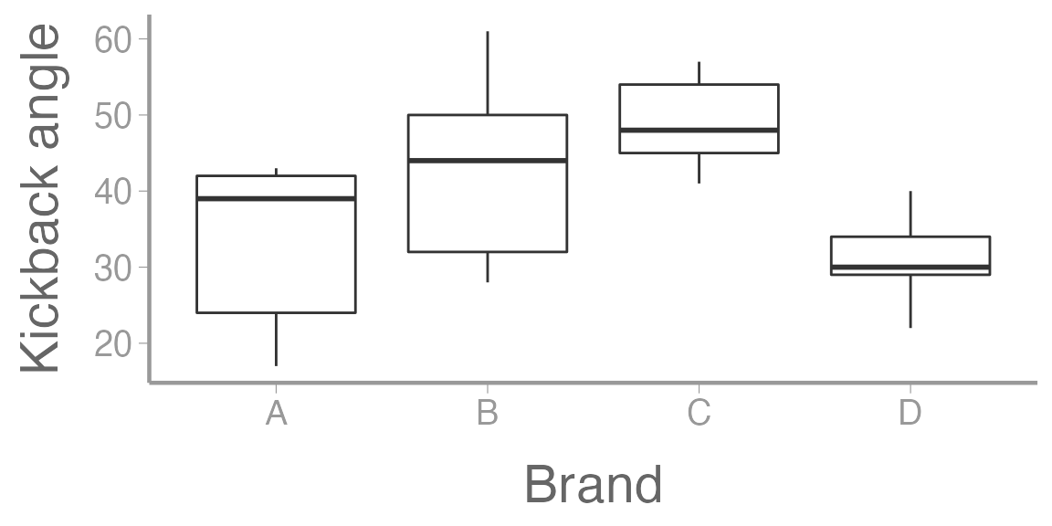
Visualize the data:
ggplot(sawData, aes(x = Brand, y = y)) +
  geom_boxplot() +
  scale_y_continuous("Kickback angle")
Using aov()
Do the analysis
aov.out1 <- aov(y ~ Brand, data = sawData)View the ANOVA table
summary(aov.out1)
#>             Df Sum Sq Mean Sq F value Pr(>F)
#> Brand        3   1080     360    3.56  0.038 *
#> Residuals   16   1620     101
#> ---
#> Signif. codes:  0 '***' 0.001 '**' 0.01 '*' 0.05 '.' 0.1 ' ' 1
The default output from summary is fine for viewing in
the console but what if you want to include the ANOVA table in a report
or paper? You could manually create a table and copy/paste the values,
but that’s a pain. Luckily, there is a handy package called
broom that turns the output from many model functions into
cleaned-up data frames:
broom::tidy(aov.out1)
#> # A tibble: 2 × 6
#>   term         df sumsq meansq statistic p.value
#>   <chr>     <dbl> <dbl>  <dbl>     <dbl>   <dbl>
#> 1 Brand         3 1080.   360.      3.56  0.0382
#> 2 Residuals    16 1620    101.     NA    NA
In R Markdown, we can even include that data frame as a nicely formatted table directly in the knitted document:
aov_df <- broom::tidy(aov.out1)

options(knitr.kable.NA = '') # don't print NA's in table
knitr::kable(aov_df,
      col.names = c("Source", "df", "SS", "MS", "F", "p"),
align = 'c', format = "html") | Source | df | SS | MS | F | p |
|---|---|---|---|---|---|
| Brand | 3 | 1080 | 360.0 | 3.556 | 0.0382 |
| Residuals | 16 | 1620 | 101.2 |
Estimates of means ( \(\mu\)’s) and SE’s
model.tables(aov.out1, type = "means", se = TRUE)
#> Tables of means
#> Grand mean
#>
#> 39
#>
#>  Brand
#> Brand
#>  A  B  C  D
#> 33 43 49 31
#>
#> Standard errors for differences of means
#>         Brand
#>         6.364
#> replic.     5
Estimates of effect sizes ( \(\alpha\)’s) and SE’s
model.tables(aov.out1, type = "effects", se = TRUE)
#> Tables of effects
#>
#>  Brand
#> Brand
#>  A  B  C  D
#> -6  4 10 -8
#>
#> Standard errors of effects
#>         Brand
#>           4.5
#> replic.     5
ANOVA by hand
Grand mean
(ybar. <- mean(sawData$y))
#> [1] 39
Group means
As with most things in R, there are several ways to
calculate the group means. First, find the group means, the hard
way:
A <- sawData$y[sawData$Brand == "A"]
B <- sawData$y[sawData$Brand == "B"]
C <- sawData$y[sawData$Brand == "C"]
D <- sawData$y[sawData$Brand == "D"]

(ybar.i <- c(mean(A), mean(B), mean(C), mean(D)))
#> [1] 33 43 49 31
Better yet, use tapply to find the group means (the base
R way):
(ybar.i <- tapply(sawData$y, INDEX = sawData$Brand, FUN = mean))
#>  A  B  C  D
#> 33 43 49 31
Finally, find the group means, the tidyverse way:
library(dplyr)
(ybar.i <- sawData %>%
            group_by(Brand) %>%
             summarise(mu = mean(y)))
#> # A tibble: 4 × 2
#>   Brand    mu
#>   <chr> <dbl>
#> 1 A        33
#> 2 B        43
#> 3 C        49
#> 4 D        31
Although each of these methods does what we want - return the mean kickback angle for each group - note that they do not return the same type of object.
Use the class() function to see what type of object each
one returns.
When might the output from each method be useful?
Sum of squares
Sums of squares among
# Number of saw brands
a <- length(unique(sawData$Brand))

# Number of measurements of each brand (note, this assumes balanced design)
n <- nrow(sawData)/a

SSa <- n * sum((ybar.i$mu - ybar.)^2)
SSa
#> [1] 1080
Sums of squares within
Multiple comparisons
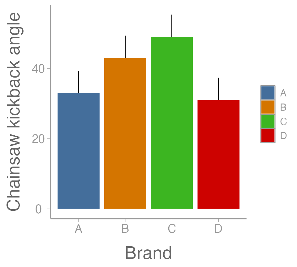
Group means +1 SE
mean.SE <- 6.364 # from model.tables() -- see slide 7.

# Add SE column
ybar.i <- dplyr::mutate(ybar.i, SE = mu + mean.SE)

ggplot(ybar.i, aes(x = Brand, y = mu, fill = Brand)) +
  geom_col() +
  geom_errorbar(aes(ymin = mu, ymax = SE), width = 0) +
  scale_y_continuous("Chainsaw kickback angle")
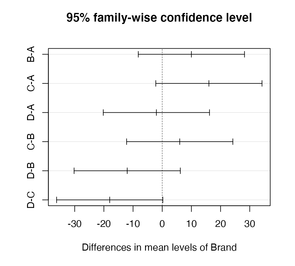
Tukey’s Honestly Significant Difference test
TukeyHSD(aov.out1)
#>   Tukey multiple comparisons of means
#>     95% family-wise confidence level
#>
#> Fit: aov(formula = y ~ Brand, data = sawData)
#>
#> $Brand
#>     diff     lwr     upr  p adj
#> B-A   10  -8.207 28.2074 0.4214
#> C-A   16  -2.207 34.2074 0.0956
#> D-A   -2 -20.207 16.2074 0.9888
#> C-B    6 -12.207 24.2074 0.7826
#> D-B  -12 -30.207  6.2074 0.2727
#> D-C -18 -36.207 0.2074 0.0532Assignment
A biologist wants to compare the growth of four different tree species she is considering for use in reforestation efforts. All 32 seedlings of the four species are planted at the same time in a large plot. Heights in meters recorded after several years.
Create an R Markdown file to do the following:
- Create an
Rchunk to load the data using:
Create a header called “Hypotheses” and under this header, indicate, in plain English, what the null and alternative hypotheses are. Also use R Markdown’s equation features to write these hypotheses (to the extent possible) using mathematical notation
Create a header called “ANOVA by hand”. Under this header, perform an ANOVA analysis (degrees of freedom, sums-of-squares, mean-squares, and F-value) without using
aov(). Compute either the critical value of F, or the p-value. Be sure to annotate your code.Create a header called “ANOVA in R”. Under this header, perform an ANOVA analysis on the data using the
aov()function-
Under a subheader called “ANOVA results”:
indicate whether or not the null hypothesis can be rejected at the \(\alpha = 0.05\) level
include a well-formatted ANOVA table using the
broom::tidy()functioncreate a barplot showing the group means and SEs
Create a header called “Which means are different?”. Use Tukey’s HSD test to determine which pairs of means differ at the \(\alpha = 0.05\) level. Include a few sentences indicating which pairs are different
A few things to remember when creating the assignment:
Be sure the output type is set to:
output: html_documentTitle the document:
title: "Homework 1"Be sure to include your first and last name in the
authorsectionBe sure to set
echo = TRUEin allRchunks so we can see both your code and the outputPlease upload both the
htmland.Rmdfiles when you submit your assignmentSee the R Markdown reference sheet for help with creating
Rchunks, equations, tables, etc.
