Lab 8: Factorial designs
FANR 6750: Experimental Methods in Forestry and Natural Resources Research
Fall 2022
lab08_factorial.RmdSituation
When do we use a factorial design? Generally, when:
There are 2 factors thought to influence the response variable
The effect of each factor might depend on the other factor
We have replicates for each combination of factors
Example: effects of food and predators on microtus voles
The data
| voles | food | predators |
|---|---|---|
| 10 | 0 | Present |
| 12 | 0 | Present |
| 8 | 0 | Present |
| 14 | 0 | Present |
| 18 | 1 | Present |
| 20 | 1 | Present |
str(microtusData)
#> 'data.frame':    24 obs. of  3 variables:
#>  $ voles    : int  10 12 8 14 18 20 21 24 20 18 ...
#>  $ food     : int  0 0 0 0 1 1 1 1 2 2 ...
#>  $ predators: chr  "Present" "Present" "Present" "Present" ...
As before, we need to convert food to a factor:
microtusData$food <- factor(microtusData$food)
str(microtusData)
#> 'data.frame':    24 obs. of  3 variables:
#>  $ voles    : int  10 12 8 14 18 20 21 24 20 18 ...
#>  $ food     : Factor w/ 3 levels "0","1","2": 1 1 1 1 2 2 2 2 3 3 ...
#>  $ predators: chr  "Present" "Present" "Present" "Present" ...
How many replicates do we have?
Visualizing the data
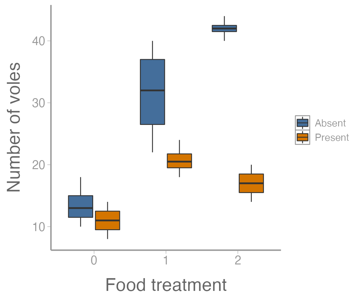
Visualizing multiple factors at once can sometimes be tricky. We’ll
use the fill aestethic to make separate boxplots for each
predation level, within each food treatment:
ggplot(microtusData, aes(x = food, y = voles, fill = predators)) +
  geom_boxplot() +
  scale_x_discrete("Food treatment") +
  scale_y_continuous("Number of voles")
It’s clear from this figure that 1) food supplementation influences vole abundance, and 2) the effects of food treatment depend on whether predators are present or absent.
Factorial design using aov()
We can analyze the microtus data using the
aov() function that we’re already familiar with. Note that
to include the interaction of food and predators, we use
food * predators in the formula:
## food * predators --> food + predators + food:predators
aov1 <- aov(voles ~ food * predators, data = microtusData)
summary(aov1)
#>                Df Sum Sq Mean Sq F value  Pr(>F)
#> food            2   1337     669    40.6 2.1e-07 ***
#> predators       1    975     975    59.2 4.3e-07 ***
#> food:predators  2    518     259    15.7 0.00011 ***
#> Residuals      18    297      16
#> ---
#> Signif. codes:  0 '***' 0.001 '**' 0.01 '*' 0.05 '.' 0.1 ' ' 1
On your own, fit the model with the interaction
(food + predators). How do the results compare?
Follow ups
Often in your own analysis, you will not stop at a significant ANOVA
result. For example, maybe you want to further explore the effects of
one factor while holding the other factor constant. In this case, we can
further test whether food supplements influence vole abundance when
predators are present using the subset argument:
summary(aov(voles ~ food,
            data = microtusData,
            subset = predators == "Present"))
#>             Df Sum Sq Mean Sq F value Pr(>F)
#> food         2  193.5    96.7    14.8 0.0014 **
#> Residuals    9   58.8     6.5
#> ---
#> Signif. codes:  0 '***' 0.001 '**' 0.01 '*' 0.05 '.' 0.1 ' ' 1
Or when predators are absent:
summary(aov(voles ~ food,
            data = microtusData,
            subset = predators == "Absent"))
#>             Df Sum Sq Mean Sq F value  Pr(>F)
#> food         2   1662     831    31.4 8.7e-05 ***
#> Residuals    9    238      26
#> ---
#> Signif. codes:  0 '***' 0.001 '**' 0.01 '*' 0.05 '.' 0.1 ' ' 1
Or maybe we want to test which levels are different using our old friend the Tukey HSD test, which for the factorial design will return both the “main” effect differences and the interaction:
TukeyHSD(aov1)
#>   Tukey multiple comparisons of means
#>     95% family-wise confidence level
#>
#> Fit: aov(formula = voles ~ food * predators, data = microtusData)
#>
#> $food
#>       diff    lwr    upr  p adj
#> 1-0 13.875  8.694 19.056 0.0000
#> 2-0 17.250 12.069 22.431 0.0000
#> 2-1  3.375 -1.806  8.556 0.2464
#>
#> $predators
#>                  diff    lwr    upr p adj
#> Present-Absent -12.75 -16.23 -9.267     0
#>
#> $`food:predators`
#>                       diff      lwr     upr  p adj
#> 1:Absent-0:Absent    18.00   8.8756  27.124 0.0001
#> 2:Absent-0:Absent    28.50  19.3756  37.624 0.0000
#> 0:Present-0:Absent   -2.50 -11.6244   6.624 0.9488
#> 1:Present-0:Absent    7.25  -1.8744  16.374 0.1684
#> 2:Present-0:Absent    3.50  -5.6244  12.624 0.8221
#> 2:Absent-1:Absent    10.50   1.3756  19.624 0.0189
#> 0:Present-1:Absent  -20.50 -29.6244 -11.376 0.0000
#> 1:Present-1:Absent  -10.75 -19.8744  -1.626 0.0158
#> 2:Present-1:Absent  -14.50 -23.6244  -5.376 0.0010
#> 0:Present-2:Absent  -31.00 -40.1244 -21.876 0.0000
#> 1:Present-2:Absent  -21.25 -30.3744 -12.126 0.0000
#> 2:Present-2:Absent  -25.00 -34.1244 -15.876 0.0000
#> 1:Present-0:Present   9.75   0.6256  18.874 0.0323
#> 2:Present-0:Present   6.00  -3.1244  15.124 0.3351
#> 2:Present-1:Present  -3.75 -12.8744   5.374 0.7781
Visualizing the results
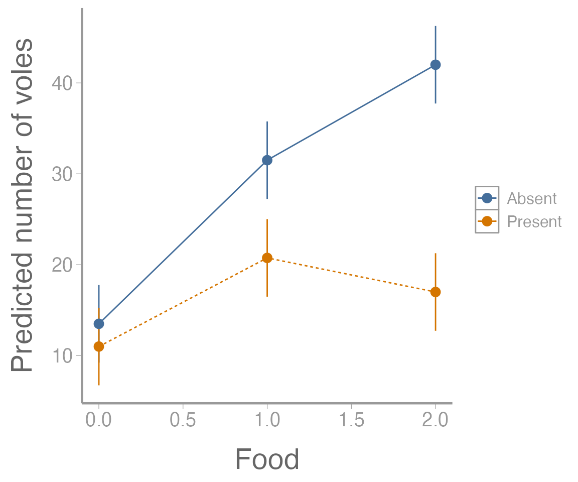
Another follow up that will often be important is visualizing the results of the ANOVA model. In the case of the factorial design, this will generally involve making a graph of the predicted response (and associated uncertainty!) for each combination of factors.
To create the data that will form the basis of this visualization,
we’ll first use the model.tables() function to compute the
relevant means (i.e., predicted values) and standard errors:
(tab <- model.tables(aov1, type="means", se = TRUE))
#> Tables of means
#> Grand mean
#>
#> 22.62
#>
#>  food
#> food
#>     0     1     2
#> 12.25 26.12 29.50
#>
#>  predators
#> predators
#>  Absent Present
#>   29.00   16.25
#>
#>  food:predators
#>     predators
#> food Absent Present
#>    0 13.50  11.00
#>    1 31.50  20.75
#>    2 42.00  17.00
#>
#> Standard errors for differences of means
#>          food predators food:predators
#>         2.030     1.658          2.871
#> replic.     8        12              4
Next, we’ll extract the group means
(ybar_ij. <- tab$tables$"food:predators")
#>     predators
#> food Absent Present
#>    0 13.50  11.00
#>    1 31.50  20.75
#>    2 42.00  17.00
What about confidence intervals? Notice that
model.tables() returns “Standard errors for differences of
means”.
Extending the formulas to the \(A \times B\) factorial case, the confidence interval for the difference in two \(A \times B\) means is:
\[\Large CI_{1−\alpha} : \bar{y}_{ij.} − \bar{y}_{ij.′} \pm t_{1−\alpha/2,ab(n−1)}\times \sqrt{\frac{2MSE}{n}}\]
where \(n = 4\) in the vole example.
To set up a plot of the group means, however, we need a confidence interval for each mean. We take out the ‘2’ from the SE expression:
\[\Large CI_{1−\alpha} : \bar{y}_{ij.} \pm t_{1−\alpha/2,ab(n−1)}\times \sqrt{\frac{MSE}{n}}\]
Where can we find MSE?
Answer: in the output of summary() of our
aov1 object:
str(summary(aov1))
#> List of 1
#>  $ :Classes 'anova' and 'data.frame':    4 obs. of  5 variables:
#>   ..$ Df     : num [1:4] 2 1 2 18
#>   ..$ Sum Sq : num [1:4] 1337 975 518 297
#>   ..$ Mean Sq: num [1:4] 668.6 975.4 259.1 16.5
#>   ..$ F value: num [1:4] 40.6 59.2 15.7 NA
#>   ..$ Pr(>F) : num [1:4] 2.15e-07 4.27e-07 1.12e-04 NA
#>  - attr(*, "class")= chr [1:2] "summary.aov" "listof"
Calculate the width of the confidence intervals:
MSE <- summary(aov1)[[1]]$`Mean Sq`[4] ## 16.5
ybar_ij.SE <- sqrt(MSE/4)
CI.half <- qt(0.975, 18) * ybar_ij.SE
(CI <- c(-CI.half, CI.half))
#> [1] -4.265  4.265
Now we can create a data frame and plot the group means and confidence intervals:
predicted.voles <- data.frame(Food = rep(c(0, 1, 2), 2),
                              Predators = rep(c("Absent", "Present"), each = 3),
                              voles = c(ybar_ij.))

## Add lower and upper confidence intervals
predicted.voles <- dplyr::mutate(predicted.voles,
                                 LCI = voles + CI[1],
                                 UCI = voles + CI[2])

## Plot results
ggplot(predicted.voles, aes(x = Food, y = voles,
                            color = Predators)) +
  geom_path(aes(linetype = Predators)) +
  geom_errorbar(aes(ymin = LCI, ymax = UCI), width = 0) +
  geom_point() +
  scale_y_continuous("Predicted number of voles")
Assignment (not for a grade)
Fictitious Scenario
Acid rain has lowered the pH of many lakes in the northeastern United States, and as a result, fish populations have declined. Managers have resorted to aerial applications of lime (powdered calcium carbonate) in hopes of increasing pH.
To determine if lime applications result in increased pH, they applied equal amounts of lime to 15 lakes, and as a control, they applied the same amount of inert white powder to an additional 15 lakes.
Researchers suspected that the effect of lime might depend upon the buffering effects of the underlying bedrock.
To assess this hypothesis, the 30 lakes were chosen such that 10 had
limestone bedrock, 10 had granite bedrock, and 10 had schist bedrock.
Acidity was measured before and after each application, and the
difference in pH is recorded in the acidityData data
set:
data("acidityData")
head(acidityData)
#>      pHdiff   bedrock treatment
#> 1  1.968718 Limestone      Lime
#> 2 -0.009063 Limestone      Lime
#> 3  1.355943 Limestone      Lime
#> 4 -0.079097 Limestone      Lime
#> 5 -1.836610 Limestone      Lime
#> 6 -1.006265 Limestone   Control
Questions/tasks
What are the null and alternative hypotheses?
Test the null hypotheses using an \(A \times B\) factorial ANOVA implemented with
aov().Does the effect of lime depend upon the bedrock type? If so, how?
Put your answers in an R Markdown report. Your report should include:
A well-formatted ANOVA table (with caption); and
A publication-quality plot of the estimated effect of lime on pH change, including 95% confidence intervals. The figure should also have a descriptive caption and any aesthetics (color, line type, etc.) should be clearly defined.
You may format the report however you like but it should be well-organized, with relevant headers, plain text, and the elements described above.
As always:
Be sure the output type is set to:
output: html_documentTitle the document:
title: "Lab 8 assignment"Be sure to include your first and last name in the
authorsectionBe sure to set
echo = TRUEin allRchunks so we can see both your code and the outputSee the R Markdown reference sheet for help with creating
Rchunks, equations, tables, etc.See the “Creating publication-quality graphics” reference sheet for tips on formatting figures