Lab 13: Linear models

Linear model review

Remember from lecture that a linear model is an equation of the form:

\[\large y_i = \beta_0 + \beta_1x_{i1} + \beta_2x_{i2} + . . . + \beta_px_{ip} + \epsilon_i\]

where the \(\beta\)’s are coefficients, and the \(x\) values are predictor variables (or dummy variables for categorical predictors).

This equation is often expressed in matrix notation as:

\[\large y = \mathbf{X\beta} + \epsilon\]

where \(X\) is a design matrix and \(\beta\) is a vector of coefficients.

The Island Scrub Jay (Aphelocoma insularis)

For this lab, we’ll use the Island Scrub Jay data from lecture:

library(FANR6750)

# Survey location/predictor data
data("cruzData")
head(cruzData)

# Jay counts
data("jayData")
head(jayData)

x	y	elevation	habitat	seeds
230737	3774324	241	Oak	Low
231037	3774324	323	Pine	Med
231337	3774324	277	Pine	High
230437	3774024	13	Oak	Med
230737	3774024	590	Oak	High
231037	3774024	533	Oak	Low

x	y	elevation	forest	chaparral	habitat	seeds	jays
258637	3764124	423	0.00	0.02	Oak	Med	34
261937	3769224	506	0.10	0.45	Oak	Med	38
246337	3764124	859	0.00	0.26	Oak	High	40
239437	3763524	1508	0.02	0.03	Pine	Med	43
239437	3767724	483	0.26	0.37	Oak	Med	36
236437	3769524	830	0.00	0.01	Oak	Low	39

The cruzData object has one row for each of the 2787 grid cell covering the island. The jayData object has counts of jays and habitat predictors for 100 (fake) survey locations.

Maps in `R`

Although we do not have time to fully cover it in this course, R has an excellent GIS and mapping capabilities. We can analyze spatial data make nice maps using a number of packages, including raster and sf. For example, we can convert the jay data to a simple features (sf) spatial object, which ggplot2 knows how to use for maps:

# Set CRS
projcrs <- "+proj=longlat +datum=WGS84 +no_defs +ellps=WGS84 +towgs84=0,0,0"

# Covert data frame to sf data frame
cruz_sf <- sf::st_as_sf(x = cruzData, coords = c("x", "y"), crs = projcrs)

# Map elevation
ggplot(cruz_sf) +
  geom_sf(aes(color = elevation), shape = 15, size = 2)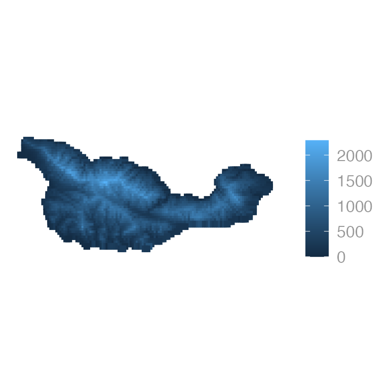

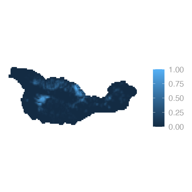
Or forest cover:

ggplot(cruz_sf) +
  geom_sf(aes(color = forest), shape = 15, size = 2)

Or chaparral with the survey locations:

jay_sf <- sf::st_as_sf(x = jayData, coords = c("x", "y"), crs = projcrs)
ggplot() +
  geom_sf(data = cruz_sf, aes(color = chaparral), shape = 15, size = 2) +
  geom_sf(data = jay_sf, color = "red")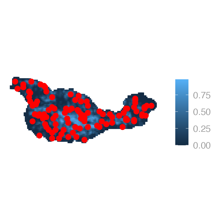

Fit some models

Simple linear regression

fm1 <- lm(jays ~ elevation, data = jayData)
summary(fm1)
#> 
#> Call:
#> lm(formula = jays ~ elevation, data = jayData)
#> 
#> Residuals:
#>    Min     1Q Median     3Q    Max 
#> -5.487 -1.754  0.157  1.616  4.615 
#> 
#> Coefficients:
#>             Estimate Std. Error t value Pr(>|t|)    
#> (Intercept) 3.31e+01   4.54e-01    72.9   <2e-16 ***
#> elevation   8.34e-03   5.95e-04    14.0   <2e-16 ***
#> ---
#> Signif. codes:  0 '***' 0.001 '**' 0.01 '*' 0.05 '.' 0.1 ' ' 1
#> 
#> Residual standard error: 2.28 on 98 degrees of freedom
#> Multiple R-squared:  0.667,  Adjusted R-squared:  0.664 
#> F-statistic:  196 on 1 and 98 DF,  p-value: <2e-16

Linear regression with quadratic effects

fm2 <- lm(jays ~ elevation + I(elevation^2), data = jayData)
summary(fm2)
#> 
#> Call:
#> lm(formula = jays ~ elevation + I(elevation^2), data = jayData)
#> 
#> Residuals:
#>    Min     1Q Median     3Q    Max 
#>  -4.84  -1.46   0.13   1.59   4.79 
#> 
#> Coefficients:
#>                 Estimate Std. Error t value Pr(>|t|)    
#> (Intercept)     3.16e+01   7.63e-01   41.43  < 2e-16 ***
#> elevation       1.37e-02   2.34e-03    5.84  6.9e-08 ***
#> I(elevation^2) -3.54e-06   1.50e-06   -2.36     0.02 *  
#> ---
#> Signif. codes:  0 '***' 0.001 '**' 0.01 '*' 0.05 '.' 0.1 ' ' 1
#> 
#> Residual standard error: 2.23 on 97 degrees of freedom
#> Multiple R-squared:  0.685,  Adjusted R-squared:  0.679 
#> F-statistic:  106 on 2 and 97 DF,  p-value: <2e-16

What is the quadratic effect measuring? How do we interpret the coefficients from this model?

Multiple linear regression

fm3 <- lm(jays ~ elevation + chaparral, data = jayData)
summary(fm3)
#> 
#> Call:
#> lm(formula = jays ~ elevation + chaparral, data = jayData)
#> 
#> Residuals:
#>    Min     1Q Median     3Q    Max 
#> -5.158 -1.578  0.023  1.532  4.600 
#> 
#> Coefficients:
#>             Estimate Std. Error t value Pr(>|t|)    
#> (Intercept) 3.28e+01   4.98e-01   65.92   <2e-16 ***
#> elevation   8.22e-03   6.02e-04   13.67   <2e-16 ***
#> chaparral   1.31e+00   1.12e+00    1.16     0.25    
#> ---
#> Signif. codes:  0 '***' 0.001 '**' 0.01 '*' 0.05 '.' 0.1 ' ' 1
#> 
#> Residual standard error: 2.28 on 97 degrees of freedom
#> Multiple R-squared:  0.672,  Adjusted R-squared:  0.665 
#> F-statistic: 99.2 on 2 and 97 DF,  p-value: <2e-16

How do we interpret the elevation and chaparral parameters in this model?

One-way ANOVA

fm4 <- lm(jays ~ habitat, data = jayData)
summary(fm4)
#> 
#> Call:
#> lm(formula = jays ~ habitat, data = jayData)
#> 
#> Residuals:
#>    Min     1Q Median     3Q    Max 
#> -7.914 -2.368 -0.368  3.086  8.632 
#> 
#> Coefficients:
#>             Estimate Std. Error t value Pr(>|t|)    
#> (Intercept)    35.88       1.36   26.46   <2e-16 ***
#> habitatOak      3.49       1.45    2.41    0.018 *  
#> habitatPine     2.04       1.50    1.36    0.178    
#> ---
#> Signif. codes:  0 '***' 0.001 '**' 0.01 '*' 0.05 '.' 0.1 ' ' 1
#> 
#> Residual standard error: 3.84 on 97 degrees of freedom
#> Multiple R-squared:  0.0713, Adjusted R-squared:  0.0521 
#> F-statistic: 3.72 on 2 and 97 DF,  p-value: 0.0277

ANCOVA

fm5 <- lm(jays ~ habitat + elevation, data = jayData)
summary(fm5)
#> 
#> Call:
#> lm(formula = jays ~ habitat + elevation, data = jayData)
#> 
#> Residuals:
#>    Min     1Q Median     3Q    Max 
#> -5.033 -1.536  0.009  1.469  4.239 
#> 
#> Coefficients:
#>             Estimate Std. Error t value Pr(>|t|)    
#> (Intercept) 3.07e+01   8.08e-01   38.00  < 2e-16 ***
#> habitatOak  3.17e+00   7.85e-01    4.03  0.00011 ***
#> habitatPine 1.70e+00   8.15e-01    2.08  0.04010 *  
#> elevation   8.29e-03   5.41e-04   15.31  < 2e-16 ***
#> ---
#> Signif. codes:  0 '***' 0.001 '**' 0.01 '*' 0.05 '.' 0.1 ' ' 1
#> 
#> Residual standard error: 2.08 on 96 degrees of freedom
#> Multiple R-squared:  0.73,   Adjusted R-squared:  0.722 
#> F-statistic: 86.6 on 3 and 96 DF,  p-value: <2e-16

One factor and continuous covariates with quadratic effects

fm6 <- lm(jays ~ habitat + elevation + I(elevation^2) + chaparral, data = jayData)
summary(fm6)
#> 
#> Call:
#> lm(formula = jays ~ habitat + elevation + I(elevation^2) + chaparral, 
#>     data = jayData)
#> 
#> Residuals:
#>    Min     1Q Median     3Q    Max 
#> -5.316 -1.430  0.017  1.380  4.067 
#> 
#> Coefficients:
#>                 Estimate Std. Error t value Pr(>|t|)    
#> (Intercept)     2.96e+01   9.99e-01   29.61  < 2e-16 ***
#> habitatOak      3.07e+00   7.79e-01    3.94  0.00015 ***
#> habitatPine     1.80e+00   8.11e-01    2.22  0.02864 *  
#> elevation       1.19e-02   2.25e-03    5.29  7.9e-07 ***
#> I(elevation^2) -2.45e-06   1.44e-06   -1.70  0.09207 .  
#> chaparral       7.89e-01   1.03e+00    0.77  0.44418    
#> ---
#> Signif. codes:  0 '***' 0.001 '**' 0.01 '*' 0.05 '.' 0.1 ' ' 1
#> 
#> Residual standard error: 2.06 on 94 degrees of freedom
#> Multiple R-squared:  0.741,  Adjusted R-squared:  0.727 
#> F-statistic: 53.8 on 5 and 94 DF,  p-value: <2e-16

Now things are getting pretty complicated. Be sure you can explain, in plain English, what each parameter represents

Let’s also take a moment to make some visualizations. For example, understanding quadratic effects is often easiest by visualizing predicted values:

First, create a sequence of values of elevation, holding other predictors constant

nd1 <- data.frame(habitat = "Oak", elevation = seq(min(jayData$elev), 
                                                   max(jayData$elev), length=100),
                  chaparral=mean(jayData$chaparral))

Next, obtain the predictions from the fitted model:

E6.elev <- predict(fm6, newdata = nd1, 
                   type = "response", 
                   se.fit = TRUE, 
                   interval = "confidence")
E6.elev <- cbind(E6.elev$fit, nd1)
head(E6.elev)
#>     fit   lwr   upr habitat elevation chaparral
#> 1 32.98 31.47 34.49     Oak     12.00    0.2407
#> 2 33.16 31.71 34.61     Oak     27.40    0.2407
#> 3 33.34 31.95 34.73     Oak     42.81    0.2407
#> 4 33.52 32.19 34.86     Oak     58.21    0.2407
#> 5 33.70 32.42 34.98     Oak     73.62    0.2407
#> 6 33.88 32.65 35.11     Oak     89.02    0.2407

And finally, make the plot:

ggplot() +
  geom_point(data = jayData, aes(x = elevation, y = jays)) +
  geom_path(data = E6.elev, aes(x = elevation, y = fit)) +
  geom_ribbon(data = E6.elev, aes(x = elevation, ymin = lwr, ymax = upr),
              fill = NA, color = "black", linetype = "longdash") +
  scale_x_continuous("Elevation") +
  scale_y_continuous("Number of Jays")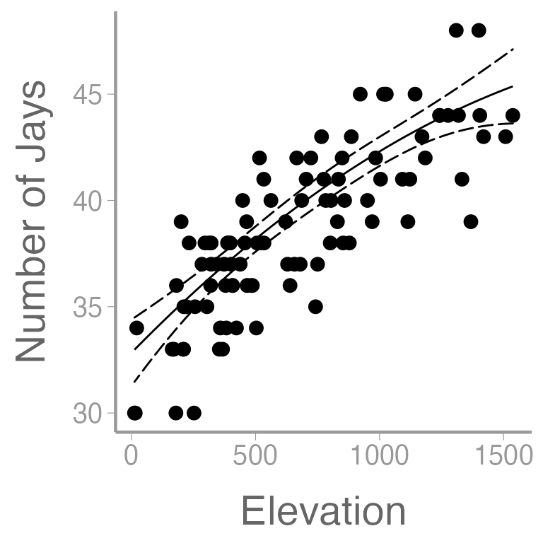

We can also predict the number of jays at each point on the entire island:

E6 <- predict(fm6, type = "response", 
              newdata = cruzData, 
              interval = "confidence")
E6 <- cbind(cruzData[,c("x","y")], E6)

E6_sf <- sf::st_as_sf(x = E6, coords = c("x", "y"), crs = projcrs)

ggplot(E6_sf) +
  geom_sf(aes(color = fit), shape = 15, size = 2) +
  scale_color_viridis_c(limits = c(30, 55)) +
  labs(title = "Expected number of Jays")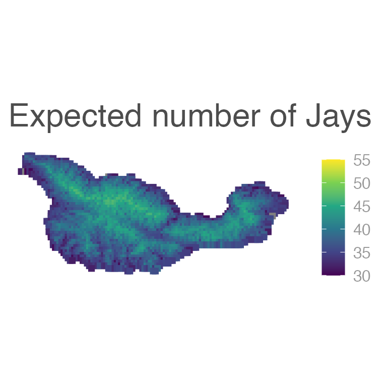

Although not often included in papers, it’s also important to show uncertainy in these predictions:

ggplot(E6_sf) +
  geom_sf(aes(color = lwr), shape = 15, size = 2) +
  scale_color_viridis_c(limits = c(30, 55)) +
  labs(title = "Lower CI")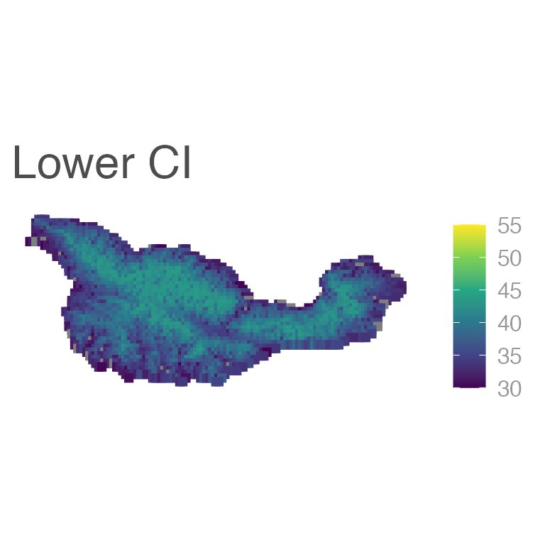

ggplot(E6_sf) +
  geom_sf(aes(color = upr), shape = 15, size = 2) +
  scale_color_viridis_c(limits = c(30, 55)) +
  labs(title = "Upper CI")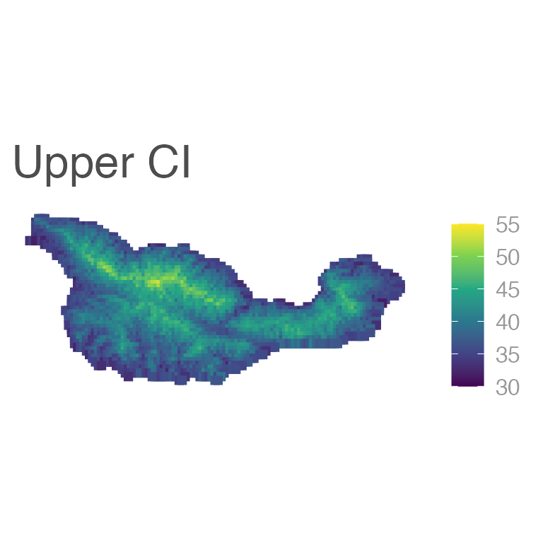

Another way to obtain the predictions

We could also obtain the predictions as follows:

X <- model.matrix(~habitat + elevation + I(elevation^2) + chaparral, data = cruzData)
beta <- coef(fm6) # beta estimates
E <- X %*% beta # expected number of jays at each pixel
head(E, n=4)
#>    [,1]
#> 1 35.38
#> 2 34.97
#> 3 34.49
#> 4 32.80

The predict() function may often be a little easier but understanding how to do obtain the predictions “by hand” like this is a good check on whether you understand 1) the design matrix, and 2) the relationship between the design matrix, model parameters, and predicted values.

Assignment: Species Richness in Switzerland

Birds are sampled at 267 locations (quadrats) as part of the Swiss breeding bird survey

The following predictor variables are available: elevation, percent cover of forest, and the presence of water

The country-wide data can be loaded using:

library(FANR6750)
data("switzerland")

The survey data can be loaded using:

data("swissData")

Create an R markdown report to do the following:

Fit 4 models of species richness using lm(). At least one model should include an interaction, and one model should include quadratic effects
Interpret, in plain English, the \(\beta\) parameter estimates for each model.
Create the design matrix for one of the models, and (matrix) multiply it by the \(\beta\) coefficients to compute the expected number of species at each plot
Use predict() to plot the relationship between expected species richness and the predictor variable with the quadratic effects. Include 95% CI in your plot.
Using the model with the interaction, predict species richness at each location in Switzerland. Include a map of the predicted values (you may use whatever graphing package you like to make the map but it must be made in R and your code must be included).

You may format the report however you like but it should be well-organized, with relevant headers, plain text, and the elements described above.

As always:

Be sure the output type is set to: output: html_document
Title the document: title: "Homework 5: Linear Regression"
Be sure to include your first and last name in the author section
Be sure to set echo = TRUE in all R chunks so we can see both your code and the output
Please upload both the html and .Rmd files when you submit your assignment
See the R Markdown reference sheet for help with creating R chunks, equations, tables, etc.
See the “Creating publication-quality graphics” reference sheet for tips on formatting figures

FANR 6750: Experimental Methods in Forestry and Natural Resources Research

Fall 2022

Linear model review

The Island Scrub Jay (Aphelocoma insularis)

Maps in `R`

Fit some models

Simple linear regression

Linear regression with quadratic effects

Multiple linear regression

One-way ANOVA

ANCOVA

One factor and continuous covariates with quadratic effects

Another way to obtain the predictions

Assignment: Species Richness in Switzerland

Lab 13: Linear models

FANR 6750: Experimental Methods in Forestry and Natural Resources Research

Fall 2022

Linear model review

The Island Scrub Jay (Aphelocoma insularis)

Maps in R

Fit some models

Simple linear regression

Linear regression with quadratic effects

Multiple linear regression

One-way ANOVA

ANCOVA

One factor and continuous covariates with quadratic effects

Another way to obtain the predictions

Assignment: Species Richness in Switzerland

Maps in `R`