Lab 6: Assumptions of ANOVA

Assumptions of the ANOVA model¹

All models have assumptions and knowing what those assumptions are, and whether our data violate any of them, is crucial to the application and interpretation of statistical models.

Before we get to the assumptions of ANOVA models, it may help to re-parameterize the model a bit. Remember from lecture that we can write the ANOVA model as:

\[\Large y_{ij} = \mu + \alpha_i + \epsilon_{ij}\]

\[\Large \epsilon_{ij} \sim normal(0, \sigma^2)\]

where

\(\mu\) is the overall mean (the horiztonal black line the below figure);
\(\alpha_i\) is the difference between the overall mean and mean of group \(i\) (the vertical orange, blue, and green, lines in the below figure);
\(\epsilon_{ij}\) is the difference between observation \(y_{ij}\) and the mean of its group (also known as residual variation; the vertical black lines in the figure); and
\(\sigma^2\) is a measure of how far, on average, each observation is from its group mean (the avarge length of the black lines in the figure).

Note that this is exactly the same as the ANOVA model, we’ve just used some basic algebra to re-write it in different terms.

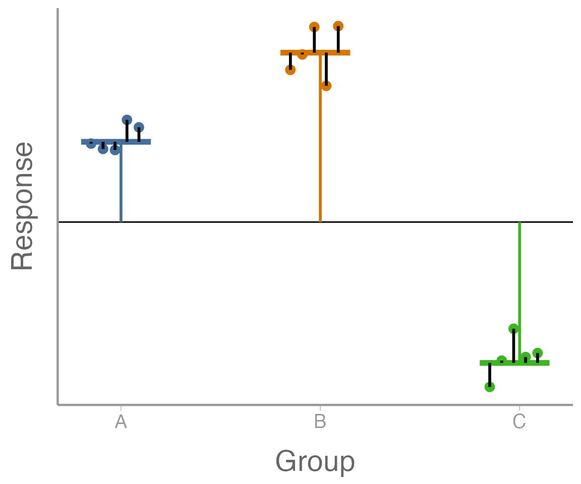
Let’s break down the above equations a bit further. First:

\[\Large E[y_{ij}] = \mu + \alpha_i\]

this says that the expected value of observation \(y_{ij}\) is \(\mu + \alpha_i\). That is, if we know what group an observation is from, this is our best guess at what value it will take. In the figure, this is the horizontal line (orange, blue, or green) for each group.

Next, we can re-write the model for observation \(y_{ij}\) as:

\[\Large y_{ij} \sim normal(E[y_{ij}], \sigma^2)\]

this says that the observations are normally distributed around the corresponding group means.

ANOVA assumptions

Now let’s look more specifically at the primary assumptions of this model:

Normality:² The ANOVA model assumes that the residuals (\(y_{ij} - E[y_{ij}]\)) are normally distributed. Note that 1) although we can formally test normality (see below), we often assess this assumption based on the nature of the data and statistical principles like the central limit theorem³, and 2) ANOVA results are pretty robust to minor violations of this assumption, so we can often trust our results even when the residuals are not normal.

Look at the equations above. Where does this assumption come from in the model?

What are some biological processes that may lead to data that violate this assumption?

Equality of variances (also known as homoscedasticity): The ANOVA model also assumes that the residual variance is the same for all groups. Another way to say this is that the residual variance is independent of group/expected value. Again, we can formally test this assumption (see lecture 3) and it’s important to do so because it is often violated.

Look at the equations above. Where does this assumption come from in the model?

What are some biological processes that may lead to data that violate this assumption?

Independence: The ANOVA model assumes that each observation \(y_{ij}\) is independent of all other observations. This is actually an assumption of virtually all models we will see this semester because it’s central to the way we calculate the likelihood of observing our data (more on this later). This assumption is a little harder to “see” in the model but it’s nonetheless there. Testing for independence is tough, so usually we assess this assumption based on our understanding of how the data were generated and observed.

What are some biological processes that may lead to data that violate this assumption?

Testing the assumptions

A fake dataset

library(FANR6750)
data("infectionRates")

str(infectionRates)
#> 'data.frame':    90 obs. of  2 variables:
#>  $ percentInfected: num  0.21 0.25 0.17 0.26 0.21 0.21 0.22 0.27 0.23 0.14 ...
#>  $ landscape      : chr  "Park" "Park" "Park" "Park" ...

summary(infectionRates)
#>  percentInfected  landscape        
#>  Min.   :0.010   Length:90         
#>  1st Qu.:0.040   Class :character  
#>  Median :0.090   Mode  :character  
#>  Mean   :0.121                     
#>  3rd Qu.:0.210                     
#>  Max.   :0.330

These data are made-up, but imagine they come from a study in which 100 crows are placed in n = 30 enclosures in each of 3 landscapes. The response variable is the proportion of crows infected with West Nile virus at the end of the study.

One-way ANOVA

anova1 <- aov(percentInfected ~ landscape, data = infectionRates)
summary(anova1)
#>             Df Sum Sq Mean Sq F value Pr(>F)    
#> landscape    2  0.638   0.319     306 <2e-16 ***
#> Residuals   87  0.091   0.001                   
#> ---
#> Signif. codes:  0 '***' 0.001 '**' 0.01 '*' 0.05 '.' 0.1 ' ' 1

Significant, but did we meet the assumptions?

Visualizing the data

library(ggplot2)

ggplot(infectionRates, aes(x = landscape, y = percentInfected)) +
  geom_boxplot() +
  scale_y_continuous("Percent infected")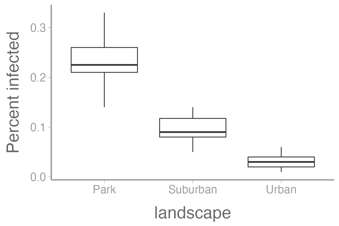

Notice that the variances don’t look equal among groups.

Visualizing the residuals

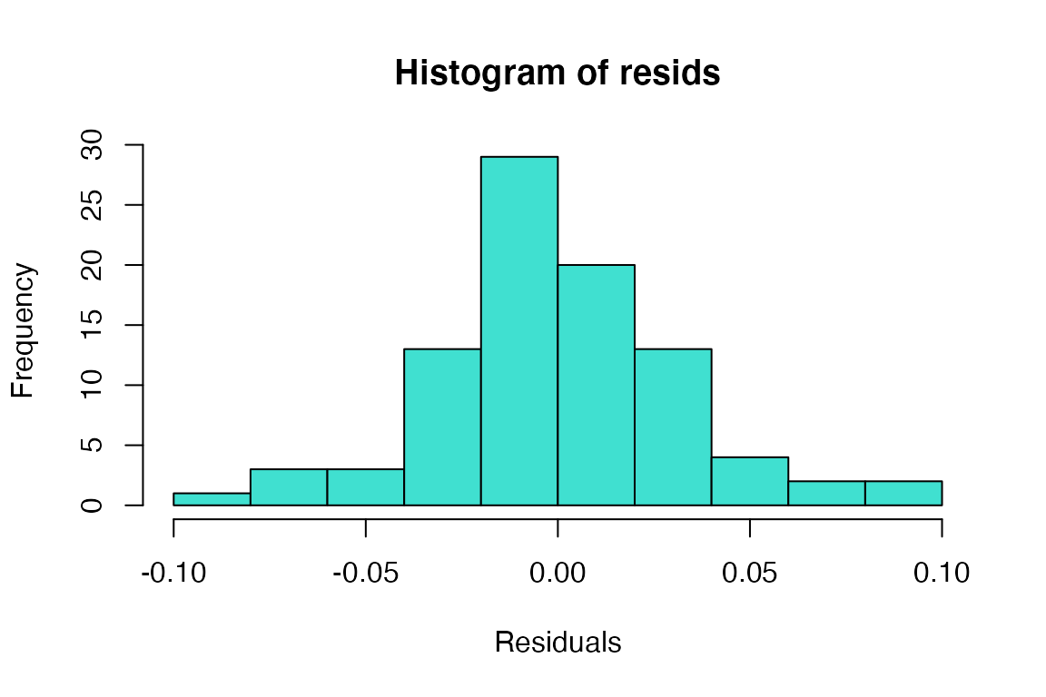
Histogram of residuals

resids <- resid(anova1)
hist(resids, col="turquoise", breaks=10, xlab="Residuals")

QQ-plot of the residuals

ggplot(anova1, aes(sample = .resid)) +
  geom_qq() +
  geom_qq_line()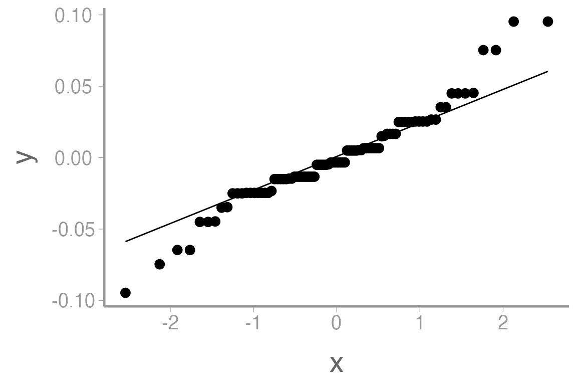

The histogram doesn’t look bad, but the QQ-plot suggests the smallest residuals are smaller than expected (below the QQ line) and the large residuals are bigger than expected (above the QQ line). We can also formally test the normality assumption using the Shapiro-Wilk test.

Normality test on residuals

shapiro.test(resids)
#> 
#>  Shapiro-Wilk normality test
#> 
#> data:  resids
#> W = 0.96, p-value = 0.004

We reject the null hypothesis that the residuals come from a normal distribution.

Clearly, we have violated both the normality and equality of variance assumptions. Since we failed to meet the key assumptions of ANOVA, we should consider transformations and/or non-parametric tests.

Transformations

One way to move forward with our analysis when assumptions are violated is to transform the response data. In some cases, simple transformations can help us meet assumptions. Knowing which transformation to use in which context requires some experience, and we have to keep in mind that the interpretation of the model parameters changes a bit. However, a good “toolkit” of standard transformations can often get you pretty far, so let’s look at a few standard choices:

Logarithmic transformation

\[\Large y = log(u + C)\]

\(y\) is the transformed response variable
\(u\) is original response variable
The constant \(C\) is often 1 if there are zeros in the data

Useful when group variances are proportional to the means

Here’s what the infection rate data looks like when log transformed:

ggplot(infectionRates, aes(x = landscape, y = log(percentInfected))) +
  geom_boxplot() +
  scale_y_continuous("log(Percent infected)")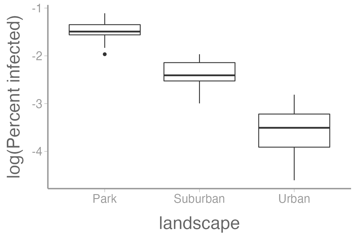

Square root transformation

\[\Large y = \sqrt{u + C}\]

\(C\) is often 0.5 or some other small number

Useful when group variances are proportional to the means

Here’s what the infection rate data looks like when square root transformed:

ggplot(infectionRates, aes(x = landscape, y = sqrt(percentInfected))) +
  geom_boxplot() +
  scale_y_continuous("sqrt(Percent infected)")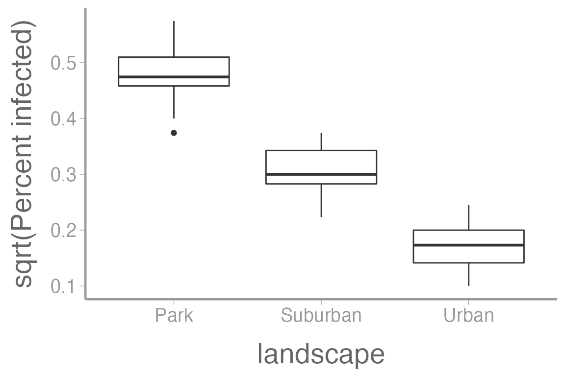

Arcsine-square root transformation

\[\Large y = arcsin(\sqrt{u})\]

logit transformation is an alternative: \(y = log\big(\frac{u}{1−u}\big)\)

Used on proportions

Here’s what the infection rate data looks like when arcsine-square root transformed:

ggplot(infectionRates, aes(x = landscape, y = asin(sqrt(percentInfected)))) +
  geom_boxplot() +
  scale_y_continuous("arcsin(sqrt(Percent infected)")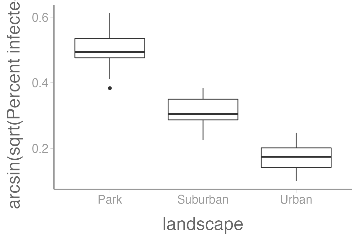

Reciprocal Transformation

\[\Large y = \frac{1}{u + C}\]

\(C\) is often 1 but could be 0 if there are no zeros in \(u\)

Useful when group SDs are proportional to the squared group means

Here’s what the infection rate data looks like when reciprocally transformed:

ggplot(infectionRates, aes(x = landscape, y = 1/(percentInfected))) +
  geom_boxplot() +
  scale_y_continuous("1/Percent infected)")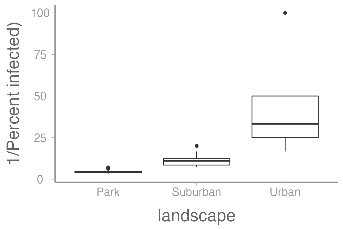

ANOVA on transformed data

Transformation can be done in the aov formula:

anova2 <- aov(log(percentInfected) ~ landscape, data = infectionRates)
summary(anova2)
#>             Df Sum Sq Mean Sq F value Pr(>F)    
#> landscape    2   60.9    30.5     304 <2e-16 ***
#> Residuals   87    8.7     0.1                   
#> ---
#> Signif. codes:  0 '***' 0.001 '**' 0.01 '*' 0.05 '.' 0.1 ' ' 1

The log transformation didn’t help much: We still reject the normality assumption

shapiro.test(resid(anova2))
#> 
#>  Shapiro-Wilk normality test
#> 
#> data:  resid(anova2)
#> W = 0.97, p-value = 0.04

Non-parametric models

Occasionally, transformations will not be sufficient or appropriate for meeting the ANOVA assumptions. In this case, we can use models that do not make assumptions about the distribution on the residuals, termed non-parametric models.

One such test is the Wilcoxan rank sum test:

For 2 group comparisons (alternative to t-test)
a.k.a. the Mann-Whitney \(U\) test
wilcox.test()

Another is the Kruskal-Wallis One-Way ANOVA

For testing differences in > 2 groups
kruskal.test()

These two functions can be used in almost the exact same way as t.test() and aov(), respectively.

Assignment

Create an R Markdown file to do the following:

Create an R chunk to load the data using:

library(FANR6750)
data("infectionRates")

Create a header called “ANOVA on transformed data”. Within this section, decide which transformation is best for the infectionRates data by conducting ANOVAs using the log, square-root, arcsine square-root, and reciprocal transformations. Use boxplots, histograms, and Shapiro’s tests to determine the best transformation.

Within this section, use subheaders to delineate different transformations. At this point in the semester, your figures should be starting to look more professional so take time to make them look nice and include captions (see fig.caption chunk option). Look over the “Creating publication-quality graphics” reference for additional tips. Also include a subheader within which you write a short conclusion about which transformation you think is best for these data.

Within the section with your conclusion about which transformation to use, discuss whether the transformation alters the conclusion about the null hypothesis of no difference in means? If not, were the transformations necessary?
Create a header called “Non-parametric test”. In this section, conduct a Kruskal-Wallis test on the data. What is the conclusion? Explain your answers.

A few things to remember when creating the assignment:

Be sure the output type is set to: output: html_document
Title the document: title: "Homework 2: Assumptions and transformations"
Be sure to include your first and last name in the author section
Be sure to set echo = TRUE in all R chunks so we can see both your code and the output
Please upload both the html and .Rmd files when you submit your assignment
See the R Markdown reference sheet for help with creating R chunks, equations, tables, etc.
See the “Creating publication-quality graphics” reference sheet for tips on formatting figures

Because we can view the t-test as a special case of an ANOVA (one with only 2 groups), these assumptions also apply to t-tests!↩︎
It’s important to note that this assumption applies to the residuals, not the response data itself. This is a common misconception↩︎
CLT↩︎

FANR 6750: Experimental Methods in Forestry and Natural Resources Research

Fall 2022

Assumptions of the ANOVA model¹

ANOVA assumptions

Testing the assumptions

A fake dataset

One-way ANOVA

Visualizing the data

Visualizing the residuals

Normality test on residuals

Transformations

Logarithmic transformation

Square root transformation

Arcsine-square root transformation

Reciprocal Transformation

ANOVA on transformed data

Non-parametric models

Assignment

Lab 6: Assumptions of ANOVA

FANR 6750: Experimental Methods in Forestry and Natural Resources Research

Fall 2022

Assumptions of the ANOVA model1

ANOVA assumptions

Testing the assumptions

A fake dataset

One-way ANOVA

Visualizing the data

Visualizing the residuals

Normality test on residuals

Transformations

Logarithmic transformation

Square root transformation

Arcsine-square root transformation

Reciprocal Transformation

ANOVA on transformed data

Non-parametric models

Assignment

Assumptions of the ANOVA model¹