Lab 12: Analysis of Covariance (ANCOVA)

Scenario

Very commonly, we are interested in doing a one-way ANOVA but we need to account for the effect of a continuous predictor variable. How do we include the continuous predictor in the ANOVA model? Analysis of covariance (ANOVA).

ANCOVA can be thought of as a hybrid between ANOVA and regression. Actually, it’s more accurate to say that ANOVA, regression, and ANCOVA are all linear models. And understanding how these models are the same, and how they differ, is critical to the application of modern statistical methods.

Example: the Diet Data

Load the data and check structure:

library(FANR6750)
data("dietData")
str(dietData)
#> 'data.frame':    60 obs. of  3 variables:
#>  $ weight: num  23.8 26 30.3 25.9 18.5 ...
#>  $ diet  : chr  "Control" "Control" "Control" "Control" ...
#>  $ length: num  11.62 13.56 15.36 7.95 5.49 ...

We need to change diet to a factor, and while doing so we’ll explicitly define the level order:

dietData$diet <- factor(dietData$diet, levels = c("Control", "Low", "Med", "High"))
levels(dietData$diet)
#> [1] "Control" "Low"     "Med"     "High"

Let’s also visualize the data:

library(ggplot2)

ggplot(dietData, aes(x = length, y = weight)) +
  geom_point()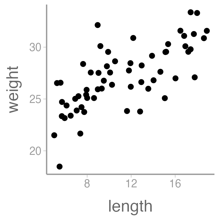


ggplot(dietData, aes(x = diet, y = weight)) +
  geom_boxplot()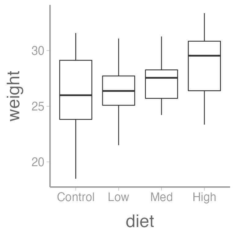

And finally, let’s quantify the relationship between length and weight using a linear regression:

fm1 <- lm(weight ~ length, dietData)
summary(fm1)

Term	Estimate	SE	Statistic	p-value
(Intercept)	21.3252	0.8069	26.430	0
length	0.5181	0.0674	7.685	0

We can also add regression lines and CIs to our plot using the predict() function:

Create a new data frame containing a sequence of values of the predictor variable length
Predict weight using these values of length
Put predictions and data together for easy plotting

lengths <- dietData$length
nd <- data.frame(length = seq(min(lengths), max(lengths), length = 50))
E1 <- predict(fm1, newdata = nd, se.fit = TRUE, interval="confidence")
predictionData <- data.frame(E1$fit, nd)

ggplot() +
  geom_point(data = dietData, aes(x = length, y = weight)) +
  geom_ribbon(data = predictionData, aes(x = length, ymin = lwr, ymax = upr),
              color = "black", linetype = "longdash", fill = NA) +
  geom_path(data = predictionData, aes(x = length, y = fit))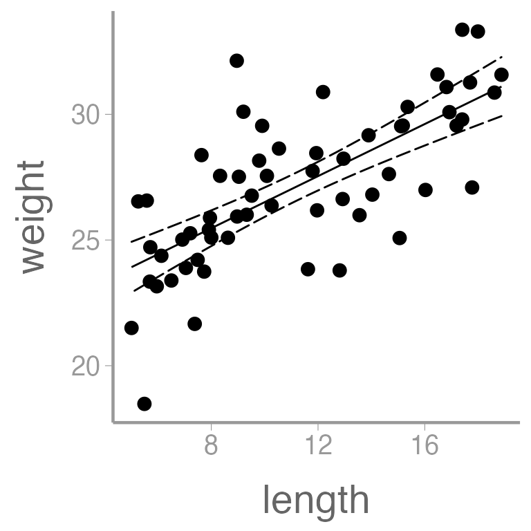

Note that in this simple case, you could use the built in stat_smooth() in ggplot2 to plot the regression line, though that will not always work. predict() is a more general method for creating and plotting regression lines from fitted models.

It’s clear that there is a strong, positive relationship between length and weight (the p-value for the slope coefficient for length is so small that R rounds it to 0). If we want to quantify whether there is an effect of diet on weight, we will clearly need to control for length in our analysis.

One-way ANOVA using `lm()`

We can also fit the conventional one-way ANOVA using lm(). We do that by changing the contrasts= argument so that the estimates will correspond to the additive model:

fm2 <- lm(weight ~ diet, dietData, contrasts = list(diet="contr.sum"))
summary.aov(fm2)
#>             Df Sum Sq Mean Sq F value Pr(>F)
#> diet         3     55   18.22    2.05   0.12
#> Residuals   56    497    8.87

As always in R, there are multiple ways to do any task. The aov() function gives identical results to the lm() function above:

summary(aov(weight ~ diet, dietData, contrasts = list(diet="contr.sum")))
#>             Df Sum Sq Mean Sq F value Pr(>F)
#> diet         3     55   18.22    2.05   0.12
#> Residuals   56    497    8.87

Note that summary() will return an alternative output compared to summary.aov():

summary(fm2)
#> 
#> Call:
#> lm(formula = weight ~ diet, data = dietData, contrasts = list(diet = "contr.sum"))
#> 
#> Residuals:
#>    Min     1Q Median     3Q    Max 
#> -7.637 -1.925 -0.037  1.977  5.458 
#> 
#> Coefficients:
#>             Estimate Std. Error t value Pr(>|t|)    
#> (Intercept)  27.1396     0.3846   70.57   <2e-16 ***
#> diet1        -1.0218     0.6661   -1.53     0.13    
#> diet2        -0.5659     0.6661   -0.85     0.40    
#> diet3         0.0803     0.6661    0.12     0.90    
#> ---
#> Signif. codes:  0 '***' 0.001 '**' 0.01 '*' 0.05 '.' 0.1 ' ' 1
#> 
#> Residual standard error: 2.98 on 56 degrees of freedom
#> Multiple R-squared:  0.0991, Adjusted R-squared:  0.0508 
#> F-statistic: 2.05 on 3 and 56 DF,  p-value: 0.117

Because we set the contrast argument to contrast="contr.sum", the intercept is the grand mean (\(\mu\)) and the other estimates are the effect sizes (\(\alpha_i\)).

Also note that you can set the behavior for all subsequent lm() or aov() calls, by setting R’s options:

options(contrasts=c("contr.sum", "contr.poly"))

And to check the value of an option:

options("contrasts")

Note that Options are reset every time you close and reopen R

As we saw earlier, the predict function can also be used to obtain group means, SEs, and CIs from a one-way ANOVA:

nd2 <- data.frame(diet=levels(dietData$diet))
E2 <- predict(fm2, newdata=nd2,
se.fit=TRUE, interval="confidence")
(predData2 <- data.frame(E2$fit, nd2))
#>     fit   lwr   upr    diet
#> 1 26.12 24.58 27.66 Control
#> 2 26.57 25.03 28.11     Low
#> 3 27.22 25.68 28.76     Med
#> 4 28.65 27.11 30.19    High

predData2$diet <- factor(predData2$diet, levels = c("Control", "Low", "Med", "High"))

ggplot(predData2) +
  geom_col(aes(x = diet, y = fit), fill = "grey50") +
  geom_errorbar(aes(x = diet, ymin = lwr, ymax = upr), width = 0.1) +
  scale_y_continuous("Weight")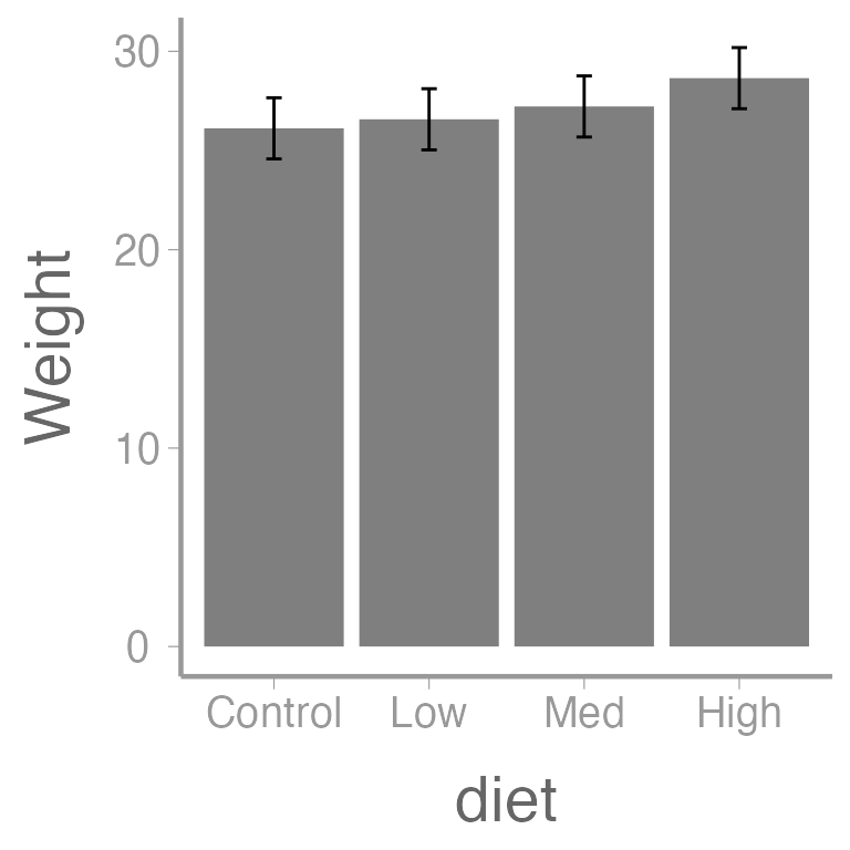

ANCOVA

Recall the additive model:

\[\Large y_{ij} = \mu + \alpha_i + \beta(x_{ij} − \bar{x}) + \epsilon_{ij}\]

Make sure the contrasts are set as before:

options(contrasts=c("contr.sum", "contr.poly"))

Centering the covariate isn’t required, but doing so allows the intercept to be interpreted as the grand mean:

dietData$lengthCentered <- dietData$length - mean(dietData$length)

Now we can fit the model using lm():

fm3 <- lm(weight ~ lengthCentered + diet, dietData)

Always put the covariate before the treatment variable in the formula. With ANCOVA, we want to assess treatment effects after accounting for the continuous covariate

Aside: Dummy variables and contrasts¹

Understanding and interpreting parameters from complex linear models can be challenging. If you are unsure about what R is doing under the hood with factors, contrasts (and interactions), a great place to start is looking at the model matrix. To do that, we need to better understand how the model matrix is constructed.

Let’s start by creating two new versions of the diet data frame. We’ll also set the factor levels and center the length data on one of the new data frames:

df <- df.orig <- dietData

df$diet <- factor(df$diet, levels = unique(df$diet))
df$length <- df$length- mean(df$length)       ###  Center df$length

Now, fit a linear model (first check the default contrasts):

options("contrasts") 
#> $contrasts
#> [1] "contr.sum"  "contr.poly"
mod1 <- lm(weight ~ length + diet, data = df, contrasts = list(diet="contr.treatment"))

And look at the estimated coefficients:

coef(mod1)
#> (Intercept)      length     dietLow     dietMed    dietHigh 
#>     25.3951      0.5573      1.3688      2.5265      3.0830

Because contr.treatment was used, (Intercept) represents the mean of the Control group, at the mean value of length (which we have set to 0).

Now let’s look at the model matrix using the model.matrix() function:

model.matrix(mod1)
#>    (Intercept)  length dietLow dietMed dietHigh
#> 1            1  0.3990       0       0        0
#> 2            1  2.3322       0       0        0
#> 3            1  4.1341       0       0        0
#> 4            1 -3.2730       0       0        0
#> 5            1 -5.7294       0       0        0
#> 6            1  7.6517       0       0        0
#> 7            1  1.5881       0       0        0
#> 8            1  6.1792       0       0        0
#> 9            1 -3.8436       0       0        0
#> 10           1  7.3886       0       0        0
#> 11           1 -5.2661       0       0        0
#> 12           1  6.5513       0       0        0
#> 13           1 -4.1749       0       0        0
#> 14           1  4.8042       0       0        0
#> 15           1  0.7117       0       0        0
#> 16           1  1.6993       1       0        0
#> 17           1  5.5913       1       0        0
#> 18           1  0.9654       1       0        0
#> 19           1 -4.7199       1       0        0
#> 20           1 -2.5990       1       0        0
#> 21           1 -0.9637       1       0        0
#> 22           1 -0.6864       1       0        0
#> 23           1  3.8912       1       0        0
#> 24           1  3.8348       1       0        0
#> 25           1 -1.7078       1       0        0
#> 26           1 -2.2548       1       0        0
#> 27           1 -6.2127       1       0        0
#> 28           1 -5.5085       1       0        0
#> 29           1  0.7417       1       0        0
#> 30           1  2.8120       1       0        0
#> 31           1 -3.2221       0       1        0
#> 32           1 -3.7347       0       1        0
#> 33           1  2.6719       0       1        0
#> 34           1 -2.8936       0       1        0
#> 35           1 -4.3085       0       1        0
#> 36           1 -5.9606       0       1        0
#> 37           1  3.9533       0       1        0
#> 38           1 -1.8963       0       1        0
#> 39           1 -5.6403       0       1        0
#> 40           1  6.4741       0       1        0
#> 41           1 -3.5908       0       1        0
#> 42           1 -1.4293       0       1        0
#> 43           1  0.5732       0       1        0
#> 44           1 -3.3137       0       1        0
#> 45           1  3.4332       0       1        0
#> 46           1 -2.2681       0       0        1
#> 47           1 -2.1892       0       0        1
#> 48           1 -1.1385       0       0        1
#> 49           1  5.2521       0       0        1
#> 50           1  5.7010       0       0        1
#> 51           1 -1.3168       0       0        1
#> 52           1  6.7679       0       0        1
#> 53           1 -5.5258       0       0        1
#> 54           1 -4.0120       0       0        1
#> 55           1 -2.0205       0       0        1
#> 56           1 -3.4903       0       0        1
#> 57           1  5.9692       0       0        1
#> 58           1 -5.0943       0       0        1
#> 59           1  6.1821       0       0        1
#> 60           1  1.7311       0       0        1
#> attr(,"assign")
#> [1] 0 1 2 2 2
#> attr(,"contrasts")
#> attr(,"contrasts")$diet
#> [1] "contr.treatment"

Remember that, in the model matrix, there is one row for each observation in the data and one column for each parameter in the model. In this case, the columns correspond to:

the intercept (= 1 for all observations)
the value of continuous covariate for each observation,
low diet
medium diet
high diet

At the bottom of print out, this function also tells you the contrasts used.

For factor levels (the final three columns in this case), the model matrix gives the values of the ‘dummy variables’ used to represent the factor diet. There will always be \(a-1\) dummy variables for a factor with a groups.

Why are there \(a-1\) dummy variables instead of \(a\)? Notice that the Control group is not in the design matrix. It has been taken as the “reference condition”: its mean is represented by the intercept. Where observations belong to the Control group, all the dummy variables have a value of 0.

To get the expected response for a particular observation, say row 1 of the data, we simply take the dot product (that is, a linear combination) of the coefficients with the appropriate row of the design matrix:

sum(coef(mod1) * model.matrix(mod1)[1,])
#> [1] 25.62
### in other words:
coef(mod1) %*% model.matrix(mod1)[1,]
#>       [,1]
#> [1,] 25.62

To do this for all rows in one go, use matrix multiplication:

coef(mod1) %*% t(model.matrix(mod1))
#>          1     2    3     4    5     6     7     8     9    10    11    12
#> [1,] 25.62 26.69 27.7 23.57 22.2 29.66 26.28 28.84 23.25 29.51 22.46 29.05
#>         13    14    15    16    17   18    19    20    21    22    23   24
#> [1,] 23.07 28.07 25.79 27.71 29.88 27.3 24.13 25.32 26.23 26.38 28.93 28.9
#>         25    26   27    28    29    30    31    32    33    34    35   36
#> [1,] 25.81 25.51 23.3 23.69 27.18 28.33 26.13 25.84 29.41 26.31 25.52 24.6
#>         37    38    39    40    41    42    43    44    45    46    47    48
#> [1,] 30.12 26.86 24.78 31.53 25.92 27.12 28.24 26.07 29.83 27.21 27.26 27.84
#>         49    50    51    52   53    54    55    56   57    58    59    60
#> [1,] 31.41 31.66 27.74 32.25 25.4 26.24 27.35 26.53 31.8 25.64 31.92 29.44

What’s with the t() function? If you’re unsure, now’s a good time to review matrix multiplication.

Next, what happens when we use contr.sum, or sum-to-zero contrasts?

mod2 <- lm(weight ~ length + diet, data = df, contrasts = list(diet="contr.sum"))

coef(mod2)
#> (Intercept)      length       diet1       diet2       diet3 
#>     27.1396      0.5573     -1.7446     -0.3758      0.7819

The (Intercept) now represents the Grand Mean (because we centered length). Also notice that the factor level now missing is High. Where did it go? Actually, we don’t need it because the effect of High can be calculated as Grand.Mean - sum(diet1, diet2, diet3).

How do you know what the intercept represents in this case? The design matrix!

model.matrix(mod2)
#>    (Intercept)  length diet1 diet2 diet3
#> 1            1  0.3990     1     0     0
#> 2            1  2.3322     1     0     0
#> 3            1  4.1341     1     0     0
#> 4            1 -3.2730     1     0     0
#> 5            1 -5.7294     1     0     0
#> 6            1  7.6517     1     0     0
#> 7            1  1.5881     1     0     0
#> 8            1  6.1792     1     0     0
#> 9            1 -3.8436     1     0     0
#> 10           1  7.3886     1     0     0
#> 11           1 -5.2661     1     0     0
#> 12           1  6.5513     1     0     0
#> 13           1 -4.1749     1     0     0
#> 14           1  4.8042     1     0     0
#> 15           1  0.7117     1     0     0
#> 16           1  1.6993     0     1     0
#> 17           1  5.5913     0     1     0
#> 18           1  0.9654     0     1     0
#> 19           1 -4.7199     0     1     0
#> 20           1 -2.5990     0     1     0
#> 21           1 -0.9637     0     1     0
#> 22           1 -0.6864     0     1     0
#> 23           1  3.8912     0     1     0
#> 24           1  3.8348     0     1     0
#> 25           1 -1.7078     0     1     0
#> 26           1 -2.2548     0     1     0
#> 27           1 -6.2127     0     1     0
#> 28           1 -5.5085     0     1     0
#> 29           1  0.7417     0     1     0
#> 30           1  2.8120     0     1     0
#> 31           1 -3.2221     0     0     1
#> 32           1 -3.7347     0     0     1
#> 33           1  2.6719     0     0     1
#> 34           1 -2.8936     0     0     1
#> 35           1 -4.3085     0     0     1
#> 36           1 -5.9606     0     0     1
#> 37           1  3.9533     0     0     1
#> 38           1 -1.8963     0     0     1
#> 39           1 -5.6403     0     0     1
#> 40           1  6.4741     0     0     1
#> 41           1 -3.5908     0     0     1
#> 42           1 -1.4293     0     0     1
#> 43           1  0.5732     0     0     1
#> 44           1 -3.3137     0     0     1
#> 45           1  3.4332     0     0     1
#> 46           1 -2.2681    -1    -1    -1
#> 47           1 -2.1892    -1    -1    -1
#> 48           1 -1.1385    -1    -1    -1
#> 49           1  5.2521    -1    -1    -1
#> 50           1  5.7010    -1    -1    -1
#> 51           1 -1.3168    -1    -1    -1
#> 52           1  6.7679    -1    -1    -1
#> 53           1 -5.5258    -1    -1    -1
#> 54           1 -4.0120    -1    -1    -1
#> 55           1 -2.0205    -1    -1    -1
#> 56           1 -3.4903    -1    -1    -1
#> 57           1  5.9692    -1    -1    -1
#> 58           1 -5.0943    -1    -1    -1
#> 59           1  6.1821    -1    -1    -1
#> 60           1  1.7311    -1    -1    -1
#> attr(,"assign")
#> [1] 0 1 2 2 2
#> attr(,"contrasts")
#> attr(,"contrasts")$diet
#> [1] "contr.sum"

Look carefully at the matrix (it might help to estimate the expected value for a few observations “by hand” to see how the dummy variables add or take away each parameters for different treatments).

So we can see that the design matrix has changed simply because we used different contrasts in the model but did the fitted values change?

all(round(coef(mod1) %*% t(model.matrix(mod1)),5) == round(coef(mod2) %*% t(model.matrix(mod2)),5))
#> [1] TRUE

Did the residuals change?

all(round(resid(mod1), 5) == round(resid(mod2), 5))
#> [1] TRUE

No indeed. Specifying different contrasts in this way is called a re-parameterization of the model. It’s a different way of doing the arithmetic of the linear model, but it comes out to the same thing. We choose a parameterization based on how we want to interpret the results. For ANOVA or ANCOVA, that’s usually sum-to-zero contrasts using contr.sum.

Back to the ANCOVA

summary(fm3)
#> 
#> Call:
#> lm(formula = weight ~ lengthCentered + diet, data = dietData)
#> 
#> Residuals:
#>    Min     1Q Median     3Q    Max 
#> -3.821 -1.221 -0.252  1.216  4.919 
#> 
#> Coefficients:
#>                Estimate Std. Error t value Pr(>|t|)    
#> (Intercept)     27.1396     0.2406  112.79  < 2e-16 ***
#> lengthCentered   0.5573     0.0594    9.38  5.2e-13 ***
#> diet1           -1.7446     0.4238   -4.12  0.00013 ***
#> diet2           -0.3758     0.4173   -0.90  0.37171    
#> diet3            0.7819     0.4234    1.85  0.07020 .  
#> ---
#> Signif. codes:  0 '***' 0.001 '**' 0.01 '*' 0.05 '.' 0.1 ' ' 1
#> 
#> Residual standard error: 1.86 on 55 degrees of freedom
#> Multiple R-squared:  0.654,  Adjusted R-squared:  0.628 
#> F-statistic: 25.9 on 4 and 55 DF,  p-value: 4.15e-12

Note that the null hypothesis of no diet effect is rejected, even though it was not rejected before.

It may also be helpful to view the ANOVA table using:

summary.aov(fm3)
#>                Df Sum Sq Mean Sq F value  Pr(>F)    
#> lengthCentered  1  278.3   278.3   80.09 2.5e-12 ***
#> diet            3   82.2    27.4    7.89 0.00018 ***
#> Residuals      55  191.1     3.5                    
#> ---
#> Signif. codes:  0 '***' 0.001 '**' 0.01 '*' 0.05 '.' 0.1 ' ' 1

And as before, we can create predictions of weight over a sequences of lengths, for every level of diet:

lengthC <- dietData$lengthCentered
nd3 <- data.frame(diet=rep(c("Control", "Low", "Med", "High"), each = 20),
                  lengthCentered=rep(seq(min(lengthC), max(lengthC),length = 20), times = 4))
E3 <- predict(fm3, newdata=nd3, se.fit = TRUE, interval = "confidence")
predData3 <- data.frame(E3$fit, nd3)

ggplot() +
  geom_point(data = dietData, aes(x = lengthCentered, y = weight, color = diet)) +
  geom_line(data = predData3, aes(x = lengthCentered, y = fit, color = diet)) +
  scale_y_continuous("Weight") +
  scale_x_continuous("Length")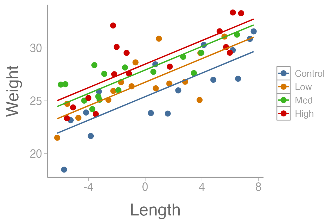

We can also look at multiple comparisons using:

library(multcomp)
summary(glht(fm3, linfct=mcp(diet="Tukey")))
#> 
#>   Simultaneous Tests for General Linear Hypotheses
#> 
#> Multiple Comparisons of Means: Tukey Contrasts
#> 
#> 
#> Fit: lm(formula = weight ~ lengthCentered + diet, data = dietData)
#> 
#> Linear Hypotheses:
#>                     Estimate Std. Error t value Pr(>|t|)    
#> Low - Control == 0     1.369      0.688    1.99   0.2038    
#> Med - Control == 0     2.526      0.697    3.62   0.0033 ** 
#> High - Control == 0    3.083      0.683    4.51   <0.001 ***
#> Med - Low == 0         1.158      0.683    1.70   0.3358    
#> High - Low == 0        1.714      0.682    2.51   0.0689 .  
#> High - Med == 0        0.557      0.687    0.81   0.8493    
#> ---
#> Signif. codes:  0 '***' 0.001 '**' 0.01 '*' 0.05 '.' 0.1 ' ' 1
#> (Adjusted p values reported -- single-step method)

Assignment (not for a grade)

Complete the following and upload your R markdown file to ELC before next week.

Fit an ANCOVA model to the treeData data set, which represent the height of trees following a fertilizer experiment. The covariate is pH.
Use sum-to-zero contrasts (contr.sum) so that your estimates correspond to the additive model from the lecture notes.
Interpret each of the estimates from lm(). What is the null hypothesis associated with each p-value?
Plot the data and the regression lines. Use different colors or symbols to distinguish the treatment groups.
Which fertilizer treatments are significantly different?

You may format the report however you like but it should be well-organized, with relevant headers, plain text, and the elements described above.

As always:

Be sure the output type is set to: output: html_document
Title the document: title: "Lab 12 optional assignment"
Be sure to include your first and last name in the author section
Be sure to set echo = TRUE in all R chunks so we can see both your code and the output
See the R Markdown reference sheet for help with creating R chunks, equations, tables, etc.
See the “Creating publication-quality graphics” reference sheet for tips on formatting figures

h/t to Bryan Nuse for this material↩︎

FANR 6750: Experimental Methods in Forestry and Natural Resources Research

Fall 2022

Scenario

Example: the Diet Data

One-way ANOVA using `lm()`

ANCOVA

Aside: Dummy variables and contrasts¹

Back to the ANCOVA

Assignment (not for a grade)

Lab 12: Analysis of Covariance (ANCOVA)

FANR 6750: Experimental Methods in Forestry and Natural Resources Research

Fall 2022

Scenario

Example: the Diet Data

One-way ANOVA using lm()

ANCOVA

Aside: Dummy variables and contrasts1

Back to the ANCOVA

Assignment (not for a grade)

One-way ANOVA using `lm()`

Aside: Dummy variables and contrasts¹