Lab 5: Contrasts, Estimation, and Power Analysis

Today’s topics

Contrasts
Estimation
Power analysis

Contrasts

Mussel data

library(FANR6750)
data("musselData")
head(musselData)
#>    Watershed Length
#> 1 Twelvemile     16
#> 2 Twelvemile      8
#> 3 Twelvemile     12
#> 4 Twelvemile     17
#> 5 Twelvemile     13
#> 6  Chattooga     18

# By default, R will order watershed in alphabetical order
# We will change it to a factor and explicitly set the order to match the order from lecture
musselData$Watershed <- factor(musselData$Watershed, 
                               levels = c("Twelvemile", "Chattooga","Keowee", "Coneross"))

Watershed	Length
Twelvemile	16
Twelvemile	8
Twelvemile	12
Twelvemile	17
Twelvemile	13
Chattooga	18

Questions

Suppose we want to make 3 a priori comparisons:

Agricultural (Twelvemile & Coneross) vs. Forested (Chattooga & Keowee)
Within agricultural (Twelvemile vs Coneross)
Within forested (Chattooga vs Keowee)

	Comparison	Null hypothesis
1	Ag. vs Forested	\(\frac{\mu_T + \mu_{Co}}{2} - \frac{\mu_{Ch} + \mu_{K}}{2} = 0\)
2	Twelvemile vs Coneross	\(\mu_T - \mu_{Co} = 0\)
3	Chattooga vs Keowee	\(\mu_{Ch} - \mu_{K} = 0\)

Constructing contrasts in R

Coefficients

AgvF <- c(1/2, -1/2, -1/2, 1/2)
TvCo <- c(1, 0, 0, -1)
ChvK <- c(0, 1, -1, 0)

Are they orthogonal?

Step 1: sum of coefficients is 0, for each contrast.

all(sum(AgvF) == 0, sum(TvCo) == 0, sum(ChvK) == 0)
#> [1] TRUE

all() tests whether all its arguments evaluate to TRUE

Step 2: pairwise dot products are all equal to 0.

all(sum(AgvF * TvCo) == 0,
    sum(AgvF * ChvK) == 0,
    sum(TvCo * ChvK) == 0)
#> [1] TRUE

Step 2 (alternate method): pairwise dot products are all equal to 0.

Try the %*% operator:

AgvF %*% TvCo
#>      [,1]
#> [1,]    0

When the operands are vectors, %*% does the dot product

Put the contrasts into a matrix

To use contrasts in R, each set of coefficients must be formatted as a column in a matrix.

We can use cbind() for this:

(contrast.mat <- cbind(AgvF, TvCo, ChvK))
#>      AgvF TvCo ChvK
#> [1,]  0.5    1    0
#> [2,] -0.5    0    1
#> [3,] -0.5    0   -1
#> [4,]  0.5   -1    0

Contrasts

Fit the model with contrasts

aov.out <- aov(Length ~ Watershed, data=musselData,
               contrasts=list(Watershed=contrast.mat))

Now partition the sum-of-squares with `split=` argument:

summary(aov.out, 
        split = list(Watershed = c("AgvF" = 1, 
                               "TvCo" = 2, 
                               "ChvK" = 3)))
#>                   Df Sum Sq Mean Sq F value  Pr(>F)    
#> Watershed          3    393     131    9.70 0.00069 ***
#>   Watershed: AgvF  1    361     361   26.76 9.2e-05 ***
#>   Watershed: TvCo  1     12      12    0.90 0.35786    
#>   Watershed: ChvK  1     20      20    1.45 0.24575    
#> Residuals         16    216      14                    
#> ---
#> Signif. codes:  0 '***' 0.001 '**' 0.01 '*' 0.05 '.' 0.1 ' ' 1

ANOVA without contrasts

\(\large F_{3, 16}\)

ANOVA with contrasts

\(\large F_{1, 16}\)

Difference in means for each contrast

Group means

library(dplyr)
(group.means <- musselData %>% 
                group_by(Watershed) %>%
                 summarise(mu = mean(Length)))
#> # A tibble: 4 × 2
#>   Watershed     mu
#>   <fct>      <dbl>
#> 1 Twelvemile  13.2
#> 2 Chattooga   21.4
#> 3 Keowee      24.2
#> 4 Coneross    15.4

Difference in means for Twelvemile vs Coneross

group.means$mu[1] - group.means$mu[4]
#> [1] -2.2

Difference in means for Chattooga vs Keowee

group.means$mu[2] - group.means$mu[3]
#> [1] -2.8

Difference in means for Ag. vs Forested

mean(group.means$mu[c(1,4)]) - mean(group.means$mu[2:3])
#> [1] -8.5

Standard errors for each contrast

SE for Twelvemile vs Coneross

se.contrast(aov.out, 
            contrast.obj = list(Watershed == "Twelvemile", Watershed == "Coneross"), 
            data = musselData)
#> [1] 2.324

SE for Chattooga vs Keowee

se.contrast(aov.out, 
            contrast.obj = list(Watershed == "Chattooga", Watershed == "Keowee"), 
            data = musselData)
#> [1] 2.324

SE for Ag. vs Forested

se.contrast(aov.out,
            contrast.obj = list(Watershed %in% c("Twelvemile","Coneross"),
                                Watershed %in% c("Chattooga","Keowee")), 
            data = musselData)
#> [1] 1.643

The %in% function returns TRUE for any elements of the first vector that match an element in the second vector and FALSE otherwise

Estimation

Estimating confidence intervals

In an ANOVA context, confidence intervals can be constructed using the equation:

\[CI = Point\; estimate \pm t_{\alpha/2,a(n−1)}\times SE\] As usual, the hard part is computing the SE

Confidence intervals from one-way ANOVA

SE’s for the effect sizes (\(\alpha\)’s)

(effects.SE <- model.tables(aov.out, type="effects", se=TRUE))
#> Tables of effects
#> 
#>  Watershed 
#> Watershed
#> Twelvemile  Chattooga     Keowee   Coneross 
#>      -5.35       2.85       5.65      -3.15 
#> 
#> Standard errors of effects
#>         Watershed
#>             1.643
#> replic.         5

Extract the \(\alpha\)’s and the SEs

# str(effects.SE)
alpha.i <- as.numeric(effects.SE$tables$Watershed)
SE <- as.numeric(effects.SE$se)

Compute confidence intervals

tc <- qt(0.975, 4 * (5 - 1))
lowerCI <- alpha.i - tc * SE
upperCI <- alpha.i + tc * SE

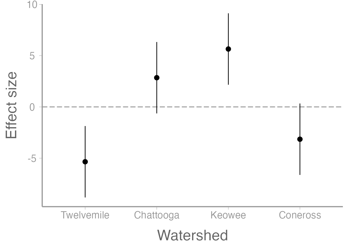
Plot effects and CIs

Put results into a data frame

CI <- data.frame(Watershed = factor(c("Twelvemile", "Chattooga",  "Keowee", "Coneross"),
                            levels = c("Twelvemile", "Chattooga","Keowee", "Coneross")),
                 effect.size = alpha.i, 
                 SE, 
                 lowerCI, 
                 upperCI)
head(CI)
#>    Watershed effect.size    SE lowerCI upperCI
#> 1 Twelvemile       -5.35 1.643 -8.8334 -1.8666
#> 2  Chattooga        2.85 1.643 -0.6334  6.3334
#> 3     Keowee        5.65 1.643  2.1666  9.1334
#> 4   Coneross       -3.15 1.643 -6.6334  0.3334

And plot:

ggplot(CI, aes(x = Watershed, y = effect.size)) +
  geom_hline(yintercept = 0, linetype = "longdash", color = "grey50") +
  geom_errorbar(aes(ymin = lowerCI, ymax = upperCI), width = 0) +
  geom_point() +
  scale_y_continuous("Effect size")

Power analysis

Statistical Power

Errors:

Type I: the null hypothesis is true, but you reject it
Type II: the null hypothesis is false, but you fail to reject it
\(\alpha = Pr(Type\;I\;error)\)
\(\beta = Pr(Type\;II\;error)\)

Power = Pr(rejecting a false null) = \(1 − \beta\)

In R functions power.t.test() and power.anova.test(), you provide all but one of the “ingredients” for the hypothesis test and determination of power. Then the missing ingredient is estimated.

Power analysis for a 2-sample t-test

power.t.test(n = NULL, 
             delta = 3, 
             sd = 2, 
             sig.level = 0.05, 
             power = 0.8)
#> 
#>      Two-sample t test power calculation 
#> 
#>               n = 8.06
#>           delta = 3
#>              sd = 2
#>       sig.level = 0.05
#>           power = 0.8
#>     alternative = two.sided
#> 
#> NOTE: n is number in *each* group

Power analysis for one-way ANOVA

power.anova.test(groups = 4, 
                 n = 5, 
                 between.var = 360.0,
                 within.var = 101.2, 
                 power = NULL)
#> 
#>      Balanced one-way analysis of variance power calculation 
#> 
#>          groups = 4
#>               n = 5
#>     between.var = 360
#>      within.var = 101.2
#>       sig.level = 0.05
#>           power = 0.9999
#> 
#> NOTE: n is number in each group

Assignment (not for a grade)

Researchers wish to know if food supplementation affects the growth of nestling Canada warblers. The treatment groups are: (A) No supplementation control, (B) low, (C) medium, (D) high, and (E) very high. The response variable is the weight of a ten-day-old nestling.

Create an R Markdown file to do the following:

Create an R chunk to load the data using:

library(FANR6750)
data("warblerWeight")

The researchers are interested in the following contrasts. Create a header called “Contrasts” and determine whether these contrasts are orthogonal. Show your work!
- Groups A,B vs C,D,E
- Groups A vs B
- Groups C vs D,E
- Groups D vs E
Create a header called “ANOVA analysis”. Under this header, use the warblerWeight data to test the null hypothesis of each contrast. This section should include a well-formatted ANOVA table showing the results of the analysis. Use the caption argument in the kable() function to include a brief caption for the ANOVA table and the round argument to print an appropriate number of digits.
In addition to the ANOVA table, compute and report, in a second table (with caption), the following for each contrast:
- The difference in the means
- The SE of the difference in means
- The 95% CI for the difference in means
Suppose you wanted to replicate the study with a smaller sample size of \(n = 2\) per treatment group. In a new section called “Power analysis”, calculate and report your power for this new experiment. This section should include both the R code you used to conduct the power analysis, and a brief (1-3 sentence) description of the result and interpretation.

A few things to remember when creating the document:

Be sure the output type is set to: output: html_document
Be sure to set echo = TRUE in all R chunks so that all code and output is visible in the knitted document
Regularly knit the document as you work to check for errors
See the R Markdown reference sheet for help with creating R chunks, equations, tables, etc.
See the “Creating publication-quality graphics” reference sheet for tips on formatting figures

FANR 6750: Experimental Methods in Forestry and Natural Resources Research

Fall 2022

Today’s topics

Contrasts

Mussel data

Questions

Constructing contrasts in R

Coefficients

Are they orthogonal?

Put the contrasts into a matrix

Contrasts

Fit the model with contrasts

Now partition the sum-of-squares with split= argument:

ANOVA without contrasts

\(\large F_{3, 16}\)

ANOVA with contrasts

\(\large F_{1, 16}\)

Difference in means for each contrast

Group means

Difference in means for Twelvemile vs Coneross

Difference in means for Chattooga vs Keowee

Difference in means for Ag. vs Forested

Standard errors for each contrast

SE for Twelvemile vs Coneross

SE for Chattooga vs Keowee

SE for Ag. vs Forested

Estimation

Estimating confidence intervals

Confidence intervals from one-way ANOVA

SE’s for the effect sizes (\(\alpha\)’s)

Extract the \(\alpha\)’s and the SEs

Compute confidence intervals

Plot effects and CIs

Put results into a data frame

And plot:

Power analysis

Statistical Power

Errors:

Power analysis for a 2-sample t-test

Power analysis for one-way ANOVA

Assignment (not for a grade)

Now partition the sum-of-squares with `split=` argument: